LotkaVolterra1.mw
Physik der sozio-ökonomischen Systeme mit dem Computer
Physics of Socio-Economic Systems with the Computer
Vorlesung gehalten an der J.W.Goethe-Universität in Frankfurt am Main (Wintersemester 2017/18)
von Dr.phil.nat. Dr.rer.pol. Matthias Hanauske
Frankfurt am Main 05.11.2017
Erster Vorlesungsteil:
Äquivalenz der
Räuber-Gleichung für N-Populationen mit der
Replikatorgleichung der evolutionären Spieltheorie für (N+1)-Strategien
Einführung
Dieses Maple-Worksheet befasst sich mit der Räuber-Beute-Gleichung für N-Populationen und berechnet deren Lösungen für den Fall N=2. Es wird ausserdem ein Bezug zwischen der Räuber-Beute-Gleichung (Lotka-Volterra Gleichung) für N-Populationen und der Replikatorgleichung der evolutionären Spieltheorie für N+1 Strategien gezogen.
| > |
restart:
with(plots):
with(plottools):
with(LinearAlgebra):
with(ColorTools):
with(StringTools): |
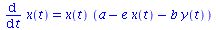
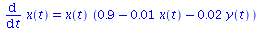
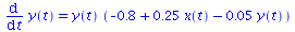
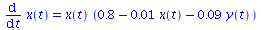
Die Räuber-Beute-Gleichung (Lotka-Volterra Gleichung) für N-Populationen (hier N=3) besteht aus dem folgenden System von Differentialgleichungen. Die Werte r[i] bezeichnen die intrinsischen Reproduktions-Sterberaten der Population i und die Matrix D_A[i,j] stellt die Interaktionsmatrix der Population i zur Population j dar (Erhöhung der Reproduktionsrate der Räuber pro Beutelebewesen bzw. Erniedriegung der Reproduktionsrate der Beutetiere pro Räuberlebewesen). Siehe z.B. Novak "Evolutionary dynamics", p.68.
| > |
Num_Pop:=3:
for i from 1 by 1 to Num_Pop do
Eqx[i]:=Dx[i]=x[i]*( r[i] + sum(D_A[i,j]*x[j],j=1..Num_Pop));
end do; |
Umschreiben des Systems:
| > |
Eqxa[1]:=subs({x[1]=x(t),x[2]=y(t),x[3]=z(t),Dx[1]=diff(x(t),t)},Eqx[1]);
Eqxa[2]:=subs({x[1]=x(t),x[2]=y(t),x[3]=z(t),Dx[2]=diff(y(t),t)},Eqx[2]);
Eqxa[3]:=subs({x[1]=x(t),x[2]=y(t),x[3]=z(t),Dx[3]=diff(z(t),t)},Eqx[3]); |
Interaktionsmatrix der Population:
| > |
D_A:=Matrix(3,3,[D_A11,D_A12,D_A13,D_A21,D_A22,D_A23,D_A31,D_A32,D_A33]); |
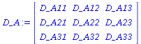 |
(1.3) |
Räuber-Beute-Gleichung für 2-Populationen (N=2)
Basierend auf Sigmund/Hofbauer S:17 ( a,b,c,d,f > 0)
| > |
D_A11:=-e:
D_A12:=-b:
D_A13:=0:
D_A21:=d:
D_A22:=-f:
D_A23:=0:
D_A31:=0:
D_A32:=0:
D_A33:=0:
r[1]:=a:
r[2]:=-c:
r[3]:=0:
print("Interaktionsmatrix");
D_A;
print("Intrinsischen Reproduktions-Sterberaten");
r[1];
r[2];
r[3]; |
System von Differentialgleichungen
 |
 |
(2.2) |
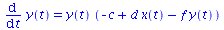
Der Fixpunkt F wird durch den Schnittpunkt der Iso-Kontourlinien diff(x(t),t)=0 und diff(y(t),t)=0 bestimmt. Falls sich die beiden Iso-Kontourlinien nicht schneiden kann eine Population aussterben.
| > |
EqFx:=subs({x(t)=x,y(t)=y},rhs(Eqxa[1])/x(t))=0;
EqFy:=subs({x(t)=x,y(t)=y},rhs(Eqxa[2])/y(t))=0;
y=solve(EqFx,y);
y=solve(EqFy,y); |
Beispiel1
| > |
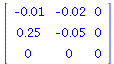
D_A11:=-0.01:
D_A12:=-0.02:
D_A13:=0:
D_A21:=0.25:
D_A22:=-0.05:
D_A23:=0:
D_A31:=0:
D_A32:=0:
D_A33:=0:
r[1]:=0.9:
r[2]:=-0.8:
r[3]:=0:
print("Interaktionsmatrix");
D_A;
print("Intrinsischen Reproduktions-Sterberaten");
r[1];
r[2];
r[3];
|
System von Differentialgleichungen
 |
 |
(2.5) |
Anfangswerte der beiden Populationen
| > |
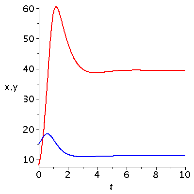
x0:=15:
y0:=8:
Loes:=dsolve({Eqxa[1],Eqxa[2],x(0)=x0,y(0)=y0},{x(t),y(t)},type=numeric,output=listprocedure); |
 |
(2.6) |
Darstellung der zeitlichen Entwicklung der Populationsvektoren (nicht normiert!). Die blaue Kurve zeigt den Beute-Populationsvektor und die rote Kurve den Räuber-Populationsvektor
| > |
tanf:=0:
tend:=10:
P1:=odeplot(Loes,[t,x(t)],tanf..tend,color=blue,axesfont=[HELVETICA,15],labelfont=[HELVETICA,15],numpoints=500,thickness=2):
P2:=odeplot(Loes,[t,y(t)],tanf..tend,color=red,axesfont=[HELVETICA,15],labelfont=[HELVETICA,15],labels=[t,"x,y"],numpoints=500,thickness=2):
display(P2,P1); |
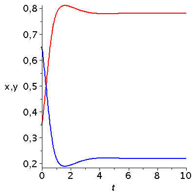
bzw. der normierten Größen:
| > |
tanf:=0:
tend:=10:
P1:=odeplot(Loes,[t,x(t)/(x(t)+y(t))],tanf..tend,color=blue,axesfont=[HELVETICA,15],labelfont=[HELVETICA,15],numpoints=500,thickness=2):
P2:=odeplot(Loes,[t,y(t)/(x(t)+y(t))],tanf..tend,color=red,axesfont=[HELVETICA,15],labelfont=[HELVETICA,15],labels=[t,"x,y"],numpoints=500,thickness=2):
display(P2,P1); |
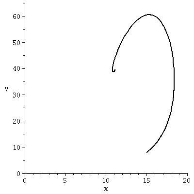
(x,y)-Populationsvektor Diagram für das Räuber-Beute Spiel:
| > |
tend:=20:
xe:=20:
ye:=65:
odeplot(Loes,[x(t),y(t)],tanf..tend,view=[0..xe,0..ye],color=black,numpoints=500,thickness=2); |
Der Fixpunkt F wird durch den Schnittpunkt der Iso-Kontourlinien diff(x(t),t)=0 und diff(y(t),t)=0 bestimmt:
| > |
EqFx:=subs({x(t)=x,y(t)=y},rhs(Eqxa[1])/x(t))=0;
EqFy:=subs({x(t)=x,y(t)=y},rhs(Eqxa[2])/y(t))=0;
y=solve(EqFx,y);
y=solve(EqFy,y); |
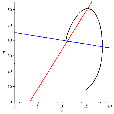
Darstellung des Fixpunktes und des (x,y)-Populationsvektors:
| > |
P1:=plot(solve(EqFx,y),x=0..xe,color=blue,view=[0..xe,0..ye],thickness=2):
P2:=plot(solve(EqFy,y),x=0..xe,color=red,view=[0..xe,0..ye],thickness=2):
P3:=odeplot(Loes,[x(t),y(t)],tanf..tend,view=[0..xe,0..ye],color=black,numpoints=500,thickness=2):
display(P3,P2,P1); |
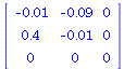
Beispiel2
| > |
D_A11:=-0.01:
D_A12:=-0.09:
D_A13:=0:
D_A21:=0.4:
D_A22:=-0.01:
D_A23:=0:
D_A31:=0:
D_A32:=0:
D_A33:=0:
r[1]:=0.8:
r[2]:=-0.5:
r[3]:=0:
print("Interaktionsmatrix");
D_A;
print("Intrinsischen Reproduktions-Sterberaten");
r[1];
r[2];
r[3]; |
System von Differentialgleichungen
 |
 |
(2.9) |
Anfangswerte der beiden Populationen
| > |
x0:=15:
y0:=8:
Loes:=dsolve({Eqxa[1],Eqxa[2],x(0)=x0,y(0)=y0},{x(t),y(t)},type=numeric,output=listprocedure); |
 |
(2.10) |
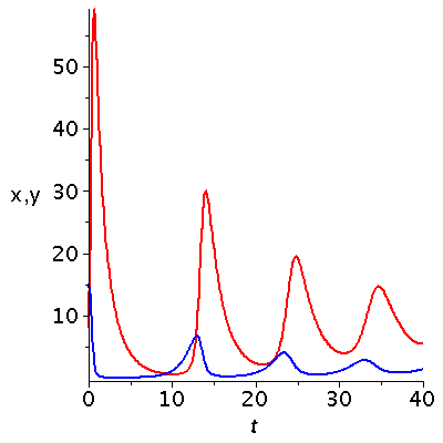
Darstellung der zeitlichen Entwicklung der Populationsvektoren (nicht normiert!). Die blaue Kurve zeigt den Beute-Populationsvektor und die rote Kurve den Räuber-Populationsvektor
| > |
tanf:=0:
tend:=40:
P1:=odeplot(Loes,[t,x(t)],tanf..tend,color=blue,axesfont=[HELVETICA,15],labelfont=[HELVETICA,15],numpoints=500,thickness=2):
P2:=odeplot(Loes,[t,y(t)],tanf..tend,color=red,axesfont=[HELVETICA,15],labelfont=[HELVETICA,15],labels=[t,"x,y"],numpoints=500,thickness=2):
display(P2,P1); |
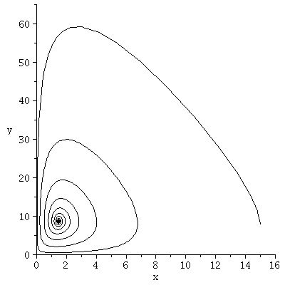
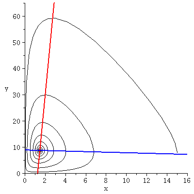
(x,y)-Populationsvektor Diagram für das Räuber-Beute Spiel:
| > |
tend:=320:
xe:=16:
ye:=65:
odeplot(Loes,[x(t),y(t)],tanf..tend,view=[0..xe,0..ye],color=black,numpoints=5000,thickness=1); |
Der Fixpunkt F wird durch den Schnittpunkt der Iso-Kontourlinien diff(x(t),t)=0 und diff(y(t),t)=0 bestimmt:
| > |
EqFx:=subs({x(t)=x,y(t)=y},rhs(Eqxa[1])/x(t))=0;
EqFy:=subs({x(t)=x,y(t)=y},rhs(Eqxa[2])/y(t))=0;
y=solve(EqFx,y);
y=solve(EqFy,y); |
Darstellung des Fixpunktes und des (x,y)-Populationsvektors:
| > |
P1:=plot(solve(EqFx,y),x=0..xe,color=blue,view=[0..xe,0..ye],thickness=2):
P2:=plot(solve(EqFy,y),x=0..xe,color=red,view=[0..xe,0..ye],thickness=2):
P3:=odeplot(Loes,[x(t),y(t)],tanf..tend,view=[0..xe,0..ye],color=black,numpoints=5000,thickness=1):
display(P3,P2,P1); |
Evolutionäre Spieltheorie und die Räuber-Beute-Gleichung (Lotka-Volterra Gleichung)
Die Räuber-Beute-Gleichung (Lotka-Volterra Gleichung) für N-Populationen lässt sich auf ein evolutionäres Spiel mit N+1 Strategien abbilden (siehe Sigmund/Hofbauer S:77 bzw. Novak "Evolutionary dynamics", p.68). Dieses Maple-Worksheet befasst sich mit dem Räuber-Beute Spiel (Anzahl der Strategien m=3 entspricht N=2 Populationen) und berechnet dessen Lösungen in einem evolutionären, zeitabhängigen Kontext.Ausgangspunkt ist eine allgemeine unsymmetrische Auszahlunsmatrix eines (2 Personen)-(3 Strategien) Spiels.
| > |
restart:
with(plots):
with(plottools):
with(LinearAlgebra):
with(ColorTools):
with(StringTools): |
Das evolutionäre Spiel besitzt folgendes System von Differentialgleichungen (Strategienanzahl 3):
| > |
Num_Strat:=3:
for i from 1 by 1 to Num_Strat do
Eqx[i]:=Dx[i]=x[i]*(sum(D_A[i,l]*x[l],l=1..Num_Strat) - sum(sum(D_A[k,l]*x[k]*x[l],k=1..Num_Strat),l=1..Num_Strat));
end do; |
Umschreiben des Systems:
| > |
Eqxa[1]:=subs({x[1]=x(t),x[2]=y(t),x[3]=1-x(t)-y(t),Dx[1]=diff(x(t),t)},Eqx[1]);
Eqxa[2]:=subs({x[1]=x(t),x[2]=y(t),x[3]=1-x(t)-y(t),Dx[2]=diff(y(t),t)},Eqx[2]);
Eqxa[3]:=subs({x[1]=x(t),x[2]=y(t),x[3]=1-x(t)-y(t),Dx[3]=diff(1-x(t)-y(t),t)},Eqx[3]); |
Definition der Auszahlunsmatrix:
| > |
D_A:=Matrix(3,3,[D_A11,D_A12,D_A13,D_A21,D_A22,D_A23,D_A31,D_A32,D_A33]); |
 |
(3.3) |
Unter Verwendung der gemischten Strategien (x,y) lässt sich eine gemischte Auszahlungsfunktion der Spieler wie folgt definieren:
| > |
Auszahlungsfunktion:=(x,y)->D_A[1,1]*x*y+D_A[1,2]*x*y+D_A[1,3]*x*(1-x-y)+D_A[2,1]*x*y+D_A[2,2]*y*y+D_A[2,3]*y*(1-x-y)+D_A[3,1]*x*(1-x-y)+D_A[3,2]*(1-x-y)*y+D_A[3,3]*(1-x-y)*(1-x-y); |
Beispiel1:
| > |
LV_D_A11:=-0.01:
LV_D_A12:=-0.02:
LV_D_A13:=0:
LV_D_A21:=0.25:
LV_D_A22:=-0.05:
LV_D_A23:=0:
LV_D_A31:=0:
LV_D_A32:=0:
LV_D_A33:=0:
r[1]:=0.9:
r[2]:=-0.8:
r[3]:=0:
print("Interaktionsmatrix");
LV_D_A;
print("Intrinsischen Reproduktions-Sterberaten");
r[1];
r[2];
r[3];
|
Die Interaktionsmatrix und die intrinsischen Reproduktions-Sterberaten sind mit der (2x3)-Spielmatrix des evolutionären Spiels in einer speziellen Weise verknüpft (siehe Sigmund/Hofbauer S:77 bzw. Novak "Evolutionary dynamics", p.68)
| > |
EqLV1:=r[1]=D_A13-D_A33;
EqLV2:=r[2]=D_A23-D_A33;
EqLV3:=LV_D_A11=D_A11-D_A31;
EqLV4:=LV_D_A12=D_A12-D_A32;
EqLV5:=LV_D_A21=D_A21-D_A31;
EqLV6:=LV_D_A22=D_A22-D_A32; |
Auflösen der Zusammenhänge
| > |
DASOLVE:=solve({EqLV1,EqLV2,EqLV3,EqLV4,EqLV5,EqLV6},{D_A11,D_A12,D_A13,D_A21,D_A22,D_A23,D_A31,D_A32}); |
Einfügen der benutzten Relationen:
| > |
Eqxaa[1]:=subs({D_A11=rhs(DASOLVE[1]),D_A12=rhs(DASOLVE[2]),D_A13=rhs(DASOLVE[3]),D_A21=rhs(DASOLVE[4]),D_A22=rhs(DASOLVE[5]),D_A23=rhs(DASOLVE[6])},Eqxa[1]);
Eqxaa[2]:=subs({D_A11=rhs(DASOLVE[1]),D_A12=rhs(DASOLVE[2]),D_A13=rhs(DASOLVE[3]),D_A21=rhs(DASOLVE[4]),D_A22=rhs(DASOLVE[5]),D_A23=rhs(DASOLVE[6])},Eqxa[2]);
Eqxaa[3]:=subs({D_A11=rhs(DASOLVE[1]),D_A12=rhs(DASOLVE[2]),D_A13=rhs(DASOLVE[3]),D_A21=rhs(DASOLVE[4]),D_A22=rhs(DASOLVE[5]),D_A23=rhs(DASOLVE[6])},Eqxa[3]); |
Das System der Differentialgleichungen vereinfacht sich durch den Befehl "simplify(...)". Beachte: Gleichungen sind jetzt unabhängig von den Auszahlungswerten der 3. Strategie:
| > |
Eqxaa[1]:=simplify(Eqxaa[1]);
Eqxaa[2]:=simplify(Eqxaa[2]);
Eqxaa[3]:=simplify(Eqxaa[3]);
|
Die Äquivalenz der Räuber-Beute-Gleichung (Lotka-Volterra Gleichung) für 2-Populationen mit der Replikatordynamik der evolutionären Spieltheorie (mit N+1 Strategien der Quasispezies) ergibt sich nun unter Verwendung des folgenden Zusammenhanges x(t)=xa(t)/(1+xa(t)+ya(t)) und y(t)=ya(t)/(1+xa(t)+ya(t)), wobei xa(t) und ya(t) die Populationsvektoren der Beute bzw. Räuber-Population repräsentieren (siehe Sigmund/Hofbauer S:77 bzw. Novak "Evolutionary dynamics", p.68).
| > |
Eqxab[1]:=simplify(expand(subs({x(t)=xa(t)/(1+xa(t)+ya(t)),y(t)=ya(t)/(1+xa(t)+ya(t))},Eqxaa[1])));
Eqxab[2]:=simplify(expand(subs({x(t)=xa(t)/(1+xa(t)+ya(t)),y(t)=ya(t)/(1+xa(t)+ya(t))},Eqxaa[2])));
Eqxab[3]:=simplify(expand(subs({x(t)=xa(t)/(1+xa(t)+ya(t)),y(t)=ya(t)/(1+xa(t)+ya(t))},Eqxaa[3]))); |
Lösung der DGL für die Anfangspopulationen aus Beispiel 1:
| > |
xa0:=15:
ya0:=8:
Loes1a:=dsolve({Eqxab[1],Eqxab[2],xa(0)=xa0,ya(0)=ya0},{xa(t),ya(t)},type=numeric,output=listprocedure); |
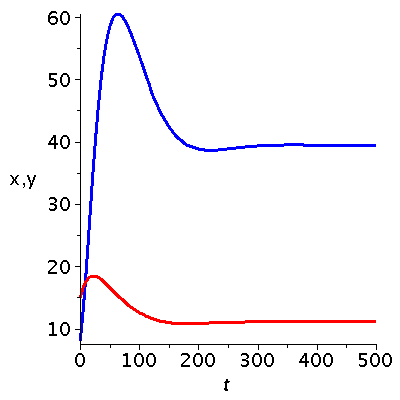
Darstellung der zeitlichen Entwicklung der Populationsvektoren:
| > |
tanf:=0:
tenda:=500:
P1:=odeplot(Loes1a,[t,xa(t)],tanf..tenda,color=red,axesfont=[HELVETICA,15],labelfont=[HELVETICA,15],numpoints=100,thickness=3):
P2:=odeplot(Loes1a,[t,ya(t)],tanf..tenda,color=blue,axesfont=[HELVETICA,15],labelfont=[HELVETICA,15],labels=[t,"x,y"],numpoints=100,thickness=3):
display(P2,P1); |
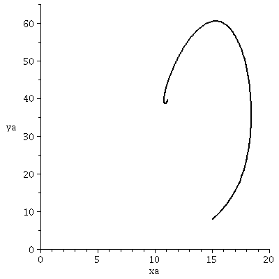
(x,y)-Populationsvektor Diagram für das Räuber-Beute Spiel:
| > |
tend:=500:
xe:=20:
ye:=65:
odeplot(Loes1a,[xa(t),ya(t)],tanf..tend,view=[0..xe,0..ye],color=black,numpoints=500,thickness=2); |
Das Bild ist identisch mit der Lösung der Lotka-Volterra Gleichun.
Beispiel 2
| > |
restart:
with(plots):
with(plottools):
with(LinearAlgebra):
with(ColorTools):
with(StringTools): |
Das evolutionäre Spiel besitzt folgendes System von Differentialgleichungen (Strategienanzahl 3):
| > |
Num_Strat:=3:
for i from 1 by 1 to Num_Strat do
Eqx[i]:=Dx[i]=x[i]*(sum(D_A[i,l]*x[l],l=1..Num_Strat) - sum(sum(D_A[k,l]*x[k]*x[l],k=1..Num_Strat),l=1..Num_Strat));
end do; |
Umschreiben des Systems:
| > |
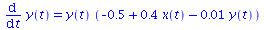
Eqxa[1]:=subs({x[1]=x(t),x[2]=y(t),x[3]=1-x(t)-y(t),Dx[1]=diff(x(t),t)},Eqx[1]);
Eqxa[2]:=subs({x[1]=x(t),x[2]=y(t),x[3]=1-x(t)-y(t),Dx[2]=diff(y(t),t)},Eqx[2]);
Eqxa[3]:=subs({x[1]=x(t),x[2]=y(t),x[3]=1-x(t)-y(t),Dx[3]=diff(1-x(t)-y(t),t)},Eqx[3]); |
Definition der Auszahlunsmatrix:
| > |
D_A:=Matrix(3,3,[D_A11,D_A12,D_A13,D_A21,D_A22,D_A23,D_A31,D_A32,D_A33]); |
 |
(3.14) |
Unter Verwendung der gemischten Strategien (x,y) lässt sich eine gemischte Auszahlungsfunktion der Spieler wie folgt definieren:
| > |
Auszahlungsfunktion:=(x,y)->D_A[1,1]*x*y+D_A[1,2]*x*y+D_A[1,3]*x*(1-x-y)+D_A[2,1]*x*y+D_A[2,2]*y*y+D_A[2,3]*y*(1-x-y)+D_A[3,1]*x*(1-x-y)+D_A[3,2]*(1-x-y)*y+D_A[3,3]*(1-x-y)*(1-x-y); |
Beispiel2:
| > |
LV_D_A11:=-0.01:
LV_D_A12:=-0.09:
LV_D_A13:=0:
LV_D_A21:=0.4:
LV_D_A22:=-0.01:
LV_D_A23:=0:
LV_D_A31:=0:
LV_D_A32:=0:
LV_D_A33:=0:
r[1]:=0.8:
r[2]:=-0.5:
r[3]:=0:
print("Interaktionsmatrix");
D_A;
print("Intrinsischen Reproduktions-Sterberaten");
r[1];
r[2];
r[3];
|
Die Interaktionsmatrix und die intrinsischen Reproduktions-Sterberaten sind mit der (2x3)-Spielmatrix des evolutionären Spiels in einer speziellen Weise verknüpft (siehe Sigmund/Hofbauer S:77 bzw. Novak "Evolutionary dynamics", p.68)
| > |
EqLV1:=r[1]=D_A13-D_A33;
EqLV2:=r[2]=D_A23-D_A33;
EqLV3:=LV_D_A11=D_A11-D_A31;
EqLV4:=LV_D_A12=D_A12-D_A32;
EqLV5:=LV_D_A21=D_A21-D_A31;
EqLV6:=LV_D_A22=D_A22-D_A32; |
| > |
DASOLVE:=solve({EqLV1,EqLV2,EqLV3,EqLV4,EqLV5,EqLV6},{D_A11,D_A12,D_A13,D_A21,D_A22,D_A23,D_A31,D_A32}); |
Einfügen der benutzten Relationen:
| > |
Eqxaa[1]:=subs({D_A11=rhs(DASOLVE[1]),D_A12=rhs(DASOLVE[2]),D_A13=rhs(DASOLVE[3]),D_A21=rhs(DASOLVE[4]),D_A22=rhs(DASOLVE[5]),D_A23=rhs(DASOLVE[6])},Eqxa[1]);
Eqxaa[2]:=subs({D_A11=rhs(DASOLVE[1]),D_A12=rhs(DASOLVE[2]),D_A13=rhs(DASOLVE[3]),D_A21=rhs(DASOLVE[4]),D_A22=rhs(DASOLVE[5]),D_A23=rhs(DASOLVE[6])},Eqxa[2]);
Eqxaa[3]:=subs({D_A11=rhs(DASOLVE[1]),D_A12=rhs(DASOLVE[2]),D_A13=rhs(DASOLVE[3]),D_A21=rhs(DASOLVE[4]),D_A22=rhs(DASOLVE[5]),D_A23=rhs(DASOLVE[6])},Eqxa[3]); |
System der Differentialgleichungen (DGL):
| > |
Eqxaa[1]:=simplify(Eqxaa[1]);
Eqxaa[2]:=simplify(Eqxaa[2]);
Eqxaa[3]:=simplify(Eqxaa[3]);
|
| > |
Eqxab[1]:=simplify(expand(subs({x(t)=xa(t)/(1+xa(t)+ya(t)),y(t)=ya(t)/(1+xa(t)+ya(t))},Eqxaa[1])));
Eqxab[2]:=simplify(expand(subs({x(t)=xa(t)/(1+xa(t)+ya(t)),y(t)=ya(t)/(1+xa(t)+ya(t))},Eqxaa[2])));
Eqxab[3]:=simplify(expand(subs({x(t)=xa(t)/(1+xa(t)+ya(t)),y(t)=ya(t)/(1+xa(t)+ya(t))},Eqxaa[3]))); |
Lösung der DGL für die Anfangspopulationen aus Beispiel 1:
| > |
xa0:=15:
ya0:=8:
Loes1a:=dsolve({Eqxab[1],Eqxab[2],xa(0)=xa0,ya(0)=ya0},{xa(t),ya(t)},type=numeric,output=listprocedure); |
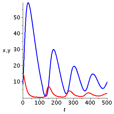
Darstellung der zeitlichen Entwicklung der Populationsvektoren:
| > |
tanf:=0:
tenda:=500:
P1:=odeplot(Loes1a,[t,xa(t)],tanf..tenda,color=red,axesfont=[HELVETICA,15],labelfont=[HELVETICA,15],numpoints=100,thickness=3):
P2:=odeplot(Loes1a,[t,ya(t)],tanf..tenda,color=blue,axesfont=[HELVETICA,15],labelfont=[HELVETICA,15],labels=[t,"x,y"],numpoints=100,thickness=3):
display(P2,P1); |
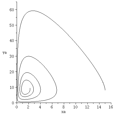
(x,y)-Populationsvektor Diagram für das Räuber-Beute Spiel:
| > |
tend:=500:
xe:=16:
ye:=65:
odeplot(Loes1a,[xa(t),ya(t)],tanf..tend,view=[0..xe,0..ye],color=black,numpoints=5000,thickness=1); |
Auch hier zeigt sich das gleiche Verhalten wie bei der Lösung der Lotka-Volterra Gleichung.