Opinion dynamics under bounded confidence
Basics of modeling opinion dynamics
Consider a group of interacting $n$ agents among whom some process of opinion formation takes place. They discuss and take opinions of others into account to a certain extent, thereby changing their opinions over time. We simplify the opinion of an agent $i$ to be some number $x_i \in [0,1]$ and the time to be discrete. Given an initial opinion profile $x(0) = (x_i(0))_{1 \le i \le n} \in S^n$ the opinion dynamics then is defined recursively by $x(t+1) = f(t, x(t))$. A simple assumption would be that $f$ is linear in the opinions $x_i(t)$ at the previous time step. Such a linear model can be modeled by different weights which an agent puts on opinions of the other agents.
Here we consider the special case where only those agents interact whose opinions differ not more than a certain confidence level $\epsilon$ (models with bounded confidence). That means, two agents do not even discuss if their opinions are split by a value greater than $\epsilon$. This may be due to a lack of understanding, a conflict of interest or social pressure. The confidence level may depend on the opinions of the two interacting agents and explicitly on the time.
Hegselmann-Krause model
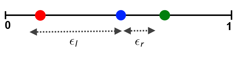
Given the opinion profile $x(t)$ and an agent $i$, the new opinion of this agent is calculated by $$ x_i(t+1) = \frac{1}{|I(i,x(t))|} \sum_{j \in I(i,x(t))} x_j(t), $$ where $I(i,x(t)) = \{1 \le i \le n: |x_j - x_i| \le \epsilon \}$ is the set of interacting agents including the agent in question himself. We put equal weights on all $j \in I(i,x)$. Instead of symmetric confidence interval $[−\epsilon, \epsilon]$, we can also consider asymmetric confidence intervals $[−\epsilon_l, \epsilon_r]$.
The original HK model can be extended by assuming that there is a true value $T$ in our opinion space $[0,1]$ which somehow attracts opinions: $$x_i(t+1) = \alpha_i T + (1 - \alpha_i) f_i(x(t)) \qquad 0 \le \alpha_i \le 1$$ Here $\alpha_i T$ is an objective component and $\alpha_i$ controls the strength of attraction to the true value. $\alpha_i$ could be interpreted as the combined effect of education, training, profession and interest. $(1 - \alpha_i) f_i(x(t))$ is the social component with $f_i(x(t)$ as defined in the original HK model. To keep things simple we assume $\alpha_i \in \{0, \alpha \}$ for all agents $i$. Agents can either be truth seekers or exclusively interact through the social component. If only a few agents are truth seekers, this is called cognitive division of labor.
Deffuant-Weisbuch model
This model uses a probabilistic approach: In each time step $t$, a pair of agents $(i,j)$ is chosen at random. The opinion of agent $i$ then changes to $$x_i(t+1) = \left\{\begin{array}{cl} \frac{1}{2} (x_i(t) + x_j(t)), & \mbox{if } -\epsilon_l \le x_j(t) - x_i(t) < \epsilon_r\\ x_i(t), & \mbox{otherwise} \end{array}\right. $$ The same applies for $i \leftrightarrow j$. This means for symmetric confidence: Agents $i$ and $j$ either agree if their opionions are within the confidence level, or they don't change their opinions at all.How to use the applet
'Start' inititializes $n$ agents with uniformly and random distributed opinions in the interval $[0,1]$. The dynamics is then calculated according to which of the radio buttons 'HK' (Hegselmann-Krause) or 'DW' (Deffuant-Weisbuch) is selected. The simulation can be stopped or paused. The simulation speed can be controlled by a slider as well as the number of agents.
There are two different types of plots. The 'time chart' plot shows the trajectories of the opinions. The opinions are spread over the vertical axis and propagate to the right over the course of the time. Each trajectory has a unique color which indicates the initial opinion. By clicking 'Show distribution' you can track the distribution of opinions at the current time. Note that the opinions are sorted in a finite number of bins, therefore it is not really a distribution. By changing the value inside the text field called 'Left bound' ('Right bound'), you can adjust the left (right) confidence level.
For the HK model, you can include a truth seeking component by adjusting the true value $T$, the strength of attraction $\alpha$ to this value, and the percentage of truth seekers.
Remarks
- Process always converges to a limit opinion profile.
- Density of limit profile: $\rho_\infty(x) = \sum_{\alpha=1}^r m_\alpha \delta(x - x_\alpha)$ with $\sum_{\alpha=1}^r m_i = 1$. $\sum_{\alpha=1}^r m_\alpha x_\alpha$ equals conserved mean opinion and all cluster fulfill $|x_\alpha - x_\beta| > \epsilon$ ($\alpha \not = \beta$) in homogeneous case.
- For further details you can take a look at the presentation and study the code.
References
- Rainer Hegselmann and Ulrich Krause. Opinion Dynamics and Bounded Confidence, Models, Analysis and Simulation. Journal of Artificial Societies and Social Simulation, 5(3):2, 2002.
- Jan Lorenz. Continuous opinion dynamics under bounded confidence: A survey. International Journal of Modern Physics C, 2007.
- Guillaume Deffuant, David Neau, Frederic Amblard, and Gerard Weisbuch. Mixing Beliefs among Interacting Agents. Advances in Complex Systems, 3:87-98, 2000.
- Rainer Hegselmann and Ulrich Krause. Truth and Cognitive Division of Labour. Journal of Artificial Societies and Social Simulation, vol. 9, no. 3. 2006.
Legal note: We do not take any responsibility for
the content of the webpages linked herein.