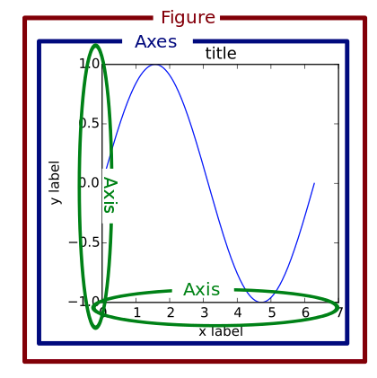
NumPy:   "numerical Python", runs in C Matplotlib:   visualization
     
#!/usr/bin/env python3
import numpy as np               # for numerics
import matplotlib.pyplot as plt  # for plotting
class globalData:      # variables are static when not declared with 'self'
 dimX = 2              # x-dimension
 dimY = 3              # y-dimension
 dimZ = 2              # y-dimension
print("*******************")
print("global data example")
print("*******************")
yxArray = np.ones( (globalData.dimY, globalData.dimX) )
zyArray = np.ones( (globalData.dimZ, globalData.dimY) )
print('yxArray :\n',yxArray)
print('zyArray :\n',zyArray)
print('zy * yx :\n',np.matmul(zyArray,yxArray))       # matrix multiplication
print("****************")
print("plotting example")
print("****************")
nPoints = 400
xPoints = range(nPoints)
yPoints = [np.sin(0.01*np.pi*x) for x in xPoints]
plt.plot(xPoints, yPoints)
plt.show()
subplots(nrows=1, ncols=1,...)
     ============================================= character description ============================================= '-' solid line style '--' dashed line style '-.' dash-dot line style ':' dotted line style '.' point marker ',' pixel marker 'o' circle marker 'v' triangle_down marker '^' triangle_up marker '<' triangle_left marker '>' triangle_right marker '1' tri_down marker '2' tri_up marker '3' tri_left marker '4' tri_right marker 's' square marker 'p' pentagon marker '*' star marker 'h' hexagon1 marker 'H' hexagon2 marker '+' plus marker 'x' x marker 'D' diamond marker 'd' thin_diamond marker '|' vline marker '_' hline marker
================== character color ================== 'b' blue 'g' green 'r' red 'c' cyan 'm' magenta 'y' yellow 'k' black 'w' white
#!/usr/bin/env python3
# importing matplotlib module
from matplotlib import pyplot as plt
from matplotlib.ticker import AutoMinorLocator
# equivalent import
# import matplotlib.pyplot as plt
 
# x-axis values
x = [5, 2, 9, 4, 7]
 
# Y-axis values
y = [10, 5, 8, 4, 2]
xMin, xMax, yMin, yMax = 2, 9, 2, 10
xTicks = range(xMin-1, xMax+2, 1)
yTicks = range(yMin  , yMax+1, 2)
 
# create figure / axis object
# quadratic outlay with figsize()
# subplots(nrows=1, ncols=1,...)
_, myAxis = plt.subplots(figsize=(10,10))
# sline are the axis / border
myAxis.spines['right'].set_linewidth(0.0)
myAxis.spines['top'].set_linewidth(0.0)
myAxis.spines['bottom'].set_linewidth(4.0)
myAxis.spines['left'].set_linewidth(4.0)
# axis start/end/labels
myAxis.axis([xMin, xMax, yMin, yMax])
myAxis.set_title('boring diagram', fontweight="bold", size=16)
myAxis.set_xlabel('x-label', fontsize = 16)
myAxis.set_ylabel('y-label', fontsize = 16) 
# major ticks by default
# minor ticks need to be activated
myAxis.tick_params(width=2, length=8, labelsize=12)
myAxis.xaxis.set_minor_locator(AutoMinorLocator())
myAxis.tick_params(which='minor', length=8, width=2, color='r')
# location of ticks
plt.setp(myAxis, xticks=xTicks, yticks=yTicks)
# plotting 
line, points = myAxis.plot(x, y, "--g",            # line
               x, y, "ob")             # points
# activate line lebel box
line.set_label('my line')
points.set_label('my points')
myAxis.legend(loc='upper center', fontsize='larger')
 
plt.show()
matplotlib.animation.FuncAnimation() 
     animation by recurrent function calling
     numpy.dtype   data type objects
#!/usr/bin/env python3
# source
# https://matplotlib.org/stable/gallery/animation/rain.html
import matplotlib.pyplot as plt
import numpy as np
from matplotlib.animation import FuncAnimation
# fixing random state for reproducibility
np.random.seed(19680801)
# create new Figure and an Axes which fills it
fig = plt.figure(figsize=(7, 7))
ax = fig.add_axes([0, 0, 1, 1], frameon=False)
ax.set_xlim(0, 1), ax.set_xticks([])
ax.set_ylim(0, 1), ax.set_yticks([])
# rain drops as an array of specified data type ´dtype'
n_drops = 50
rain_drops = np.zeros(n_drops, dtype=[('position', float, (2,)),
                                      ('size',     float),
                                      ('growth',   float),
                                      ('color',    float, (4,))])
# random initial raindrops 
rain_drops['position'] = np.random.uniform(0, 1, (n_drops, 2))
rain_drops['growth'] = np.random.uniform(50, 200, n_drops)
# scatter plot, will be updated during animation
scat = ax.scatter(rain_drops['position'][:, 0], rain_drops['position'][:, 1],
                  s=rain_drops['size'], lw=0.5, edgecolors=rain_drops['color'],
                  facecolors='none')
#
# -- the update function
#
def update(frame_number):
# get an index which we can use to re-spawn the oldest raindrop
    current_index = frame_number % n_drops
# make all colors more transparent as time progresses
    rain_drops['color'][:, 3] -= 1.0/len(rain_drops)
    rain_drops['color'][:, 3] = np.clip(rain_drops['color'][:, 3], 0, 1)
# make circles bigger
    rain_drops['size'] += rain_drops['growth']
# pick a new position for oldest rain drop, 
# resetting its size
    rain_drops['position'][current_index] = np.random.uniform(0, 1, 2)
    rain_drops['size'][current_index] = 5
    rain_drops['color'][current_index] = (0, 0, 0, 1)
    rain_drops['growth'][current_index] = np.random.uniform(50, 200)
# update the scatter collection, with the new colors, sizes and positions
    scat.set_edgecolors(rain_drops['color'])
    scat.set_sizes(rain_drops['size'])
    scat.set_offsets(rain_drops['position'])
#
# --- animation, with the update function as the animation director
#
animation = FuncAnimation(fig, update, interval=10, save_count=100)
plt.show()
#!/usr/bin/env python3
import numpy as np
import math
import matplotlib.pyplot as plt
# global parameters
nData = 2000                     # number of training pairs
nIter = 2000                     # number training iterations
nPar  =    4                     # number of fit parameters
learning_rate = 0.5e-2/nData     # relative learning rate
fitPar = []                      # empty list; fit parameters
for i in range(nPar):
  fitPar.append(np.random.randn())  
print(fitPar)
# fitting fuction
def fitFunction(x):
  sum = 0.0
  for i in range(nPar):
    sum += fitPar[i]*(x**i)
  return sum
# linespace returns a list
# training data: y= sin(x)
x = np.linspace(-math.pi, math.pi, nData)
y = np.sin(x)
# training iteration 
for iIter in range(nIter):
  y_pred = fitFunction(x)                  # list; element-wise
  loss = np.square(y_pred - y).sum()       # sum of squared elements
  if iIter % 100 == 99:                    # test printou
    print(f'{iIter:5d}  {loss:10.6f}')
  grad_y_pred = 2.0 * (y_pred - y)         # error signal
  for i in range(nPar):
    gradient = ( grad_y_pred*(x**i) ).sum()
    fitPar[i] -= learning_rate * gradient
# showing result
plt.plot(x, np.sin(x)                , 'b', label="sin(x)")
plt.plot(x, fitFunction(x)           , 'r', label="fit")
plt.plot(x, 0.0*x                    , '--k')
plt.legend()
plt.show()
#!/usr/bin/env python3
import numpy as np
x = np.array([0, 0, 1, 1, 2, 2])
y = np.array([8, 7, 6, 5, 3, 2])
z = np.array([[0, 6],
              [1, 7],
              [2, 8],
              [3, 9]])
print("\nx[:3]    ", x[:3])                # first 3 elements
print("\ny[] %    ", y[int(0.8*len(y)):])  # last 20%
print("\ny[::2]   ", y[::2])               # every second entry
print("\nx!=0     ", x!=0)                 # boolean array
print("\ny[x!=0]  ", y[x!=0])              # filtering
print("\n****************************")
print(z)
print("\nz[:,0]   ", z[:,0])               # only for np arrays
print("\nz[:,1]   ", z[:,1])
numpy.sqrt(numpy.sum(numpy.square(numPyArray)))
      numpy.linalg.norm(numPyArray) 
     numpy.sqrt(aa) = aa**2
       shortcut numpy.arange()  
#!/usr/bin/env python3
import time           # time in seconds
import numpy as np    # NumPy
NN = int(1e7)         # summing NN squares
#
# --- plain Python implementation
#
start_time = time.time()
result_plain = sum([i**2 for i in range(1, NN+1)])
end_time = time.time()
print(f"plain python, result: {result_plain:20.12e}")
print(f"plain python, time  : {end_time - start_time:7.3f}  seconds")
print()
#
# --- NumPy implementation
#
start_time = time.time()
result_numPy = \
  np.sum(np.arange(1, NN+1, dtype=np.float64)**2, dtype=np.float64)
end_time = time.time()
print(f"NumPy,        result: {result_numPy:20.12e}")
print(f"NumPy,        time  : {end_time - start_time:7.3f}  seconds")
| scipy.io | file input/output | 
| scipy.special | special functions | 
| scipy.linalg | linerar algebra | 
| scipy.interpolate | interpolations | 
| scipy.optimize | optimization and fitting | 
| scipy.stats | statistics and random numbers | 
| scipy.integrate | numerical integration | 
| scipy.fftpack | fast fourier transform | 
| scipy.signal | signal processing | 
| scipy.ndimage | image manipulation | 
#!/usr/bin/env python3
from scipy import linalg
import numpy as np
#square matrix
squareMatrix = np.array([ [5,4], [1,2] ])
print()
print("original / transposed matrix")
print(squareMatrix)
print(squareMatrix.T)
print()
#pass values to det() function
print("determinant    ", linalg.det(squareMatrix))
print()
# inverse 
print("inverse / inverse*matrix")
print(linalg.inv(squareMatrix))
print(squareMatrix.dot(linalg.inv(squareMatrix)))     # matrix multiplication
print()
#eigenvalues and vectors (as complex numbers)
print("eigenvalues | vectors")
eigenValues, eigenVectors = linalg.eig(squareMatrix)  # returning both
for ii in range(N:=len(eigenValues)):
  print(f'{ii:3d}  {np.real(eigenValues[ii]):7.4f} | ', end="")
  for jj in range(N):
    print(f'  {np.real(eigenVectors[ii][jj]):7.4f}', end="")
  print()
import datetime
print("date   today    : ", datetime.date.today())
from datetime import date
print("date   today    : ", date.today())
#!/usr/bin/env python3
import os                       # operating system
import math                     # nomen est omen
import random                   # idem
import statistics
from datetime import date
print(os.getcwd())              # current working directory
os.system('ls')                 # execute 'ls' command
if  1==2 :
  os.system('mkdir myDir')      # execute 'mkdir'
  os.chdir('myDir')             # change working directory
  os.system('cp ../test.py .')  # copy
  os.system('./test.py')        # run script (yourself again)
print()
print("math   cos      : ", math.cos(math.pi/4)*math.sqrt(2.0))
print("math   log      : ", math.log(1024, 2))
print()
print("random choice   : ", random.choice(['apple', 'pear', 'banana']))
print("random sample   : ", random.sample(range(100), 4))
print("random random   : ", random.random())
print()
data = [2.75, 1.75, 1.25, 0.25, 0.5, 1.25, 3.5]
print("stat   mean     : ", statistics.mean(data))
print("stat   variance : ", statistics.variance(data))
| namedtuple() | tuples with named fields | 
| deque | two-headed list-like container with appends and pops on either end | 
| ChainMap | dictionary-like class for creating a single view of multiple mappings | 
| Counter | dictionary subclass for counting hashable objects | 
| OrderedDict | dictionary subclass that remembers the order entries were added | 
| defaultdict | dict subclass that allows to supply missing values | 
| UserDict | wrapper around dictionary objects for easier dict subclassing | 
| UserList | wrapper around list objects for easier list subclassing | 
| UserString | wrapper around string objects for easier string subclassing | 
jupyter notebook   after installation
     virtualenv  projectDir                make one 
     source      projectDir/bin/activate   activate 
     pip install jupyter                   install, inside
     pip install matplotlib                if used, etc. 
     jupyter     notebook                  run notebook 
     for i in range(n:=5): n = n-1 print(print(i,n)) # output?