Machine Learning Primer -- Python Tutorial
Claudius Gros, WS 2025/26
Institut für theoretische Physik
Goethe-University Frankfurt a.M.
Boltzmann Machines
statistical physics
- binary neurons $ \qquad y_i\quad\to\quad s_i = -1/1$
: inactive/active
: akin to spins (physics)
- stochastic probability to flip a spin
energy functional
$$
E = -\frac{1}{2}\sum_{i,j} w_{ij} \, s_i \, s_j -
\sum_i h_i \, s_i
$$
- factor $ \ \ 1/2 \ \ $ for double counting
- magnetic field $\ \ h_i \ \ $ corresponds to $\ \ -b_i \ \ $ (threshold)
Boltzmann factor
- thermal equilibrium, temperature $\ \ T$
- probability to occupy state $\ \ \alpha=\{s_j\}$
$$
\fbox{$\phantom{\big|}\displaystyle
p_\alpha = \frac{\mbox{e}^{-\beta E_\alpha}}{Z}
\phantom{\big|}$}\,,
\qquad\quad
Z = \sum_{\alpha'} \mbox{e}^{-\beta E_{\alpha'}},
\qquad\quad
\beta=\frac{1}{k_B T}\ \to\ 1
$$
- partition function $\ \ Z$
Metropolis sampling
detailed balance
- stochastic sampling of partition function via a
random walk through configuration space
:: Monte-Carlo / Metropolis sampling
$$
p_\alpha P(\alpha\to\beta) = p_\beta P(\beta\to\alpha),
\qquad\quad
\fbox{$\phantom{\big|}\displaystyle
\frac{P(\alpha\to\beta)}{P(\beta\to\alpha)} =
\frac{p_\beta}{p_\alpha} =
\mbox{e}^{E_\alpha-E_\beta}
\phantom{\big|}$}
$$
- $P(\alpha\to\beta)\ $ probability of
selecting $\ \beta$
when in being in state $\ \alpha$
- detail balance fulfilled
$$
P(\alpha\to\beta)= \frac{\mbox{e}^{-E_\beta}}{
\mbox{e}^{-E_\alpha}+\mbox{e}^{-E_\beta}}
= \frac{1}{1+\mbox{e}^{\,E_\beta-E_\alpha}}
$$
Glauber dynamics
$$
E_\beta -E_\alpha =
\left(\frac{1}{2}\sum_{i,j} w_{ij} \, s_i \, s_j + \sum_i h_i \, s_i \right)_\alpha
-\left(\frac{1}{2}\sum_{i,j} w_{ij} \, s_i \, s_j + \sum_i h_i \, s_i \right)_\beta
$$
$\qquad$ for $\ \ \def\arraystretch{1.3} \begin{array}{r|l}
\mbox{in}\ \alpha & \mbox{in}\ \beta\\ \hline
s_k & -s_k \end{array}$
- terms $\ \ w_{ij} \, s_i \, s_j \ \ $ compensate if $\ \ i,j\ne k$
$$
\fbox{$\phantom{\big|}\displaystyle
E_\beta -E_\alpha = \epsilon_ks_k
\phantom{\big|}$}\,,
\qquad\quad
\epsilon_k = 2h_k +\sum_j w_{kj}s_j +\sum_i w_{ik}s_i
$$
- here $\ \ w_{ii}=0$
- often symmetric weights $\ \ w_{ij}=w_{ji}$
- single spin flips not used in physics (critical slowing down)
: stochastic series expansion (loop algorithm)
Boltzmann machines
2024 physics Nobel prize; Geoff Hinton
purpose
- $N_d\ $ training data $\ \ \mathbf{s}_\alpha$
- goal
maximize the probality to visit the training data
$$
\prod_{\alpha\in\mathrm{data}} p_\alpha =
\exp\left(\sum_{\alpha\in\mathrm{data}}\log(p_\alpha)\right),
\qquad\quad
\log(p_\alpha)\ : \ \mathrm{log-likelihood}
$$
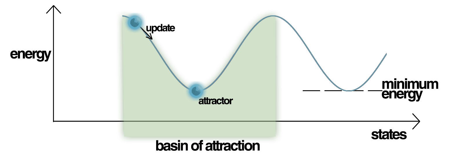
- equivalence
data configurations $\ \mathbf{s}_\alpha \ $
should be
attracting fixed points of the Glauber
dynamics
- in terms of the cross-correlation function
$$ \big\langle s_i s_j \big\rangle_{\mathrm{thermal}}
\quad\to\quad
\big\langle s_is_j\big\rangle_{\mathrm{data}}
$$
- learning is unsupervised (no explicit classifier)
Hopfield network
2024 physics Nobel prize; John Hopfield
data ↔ memories
- similar to Boltzmann machines, predecessor
- weights set by hand, not learned,
as covariance matrix of data
$$
w_{ij} = \frac{1}{N_d} \sum_{\alpha\in\mathrm{data}}
\big((\mathbf{s}_\alpha)_i- \langle s_i\rangle\big)
\big((\mathbf{s}_\alpha)_j- \langle s_j\rangle\big)
$$
- case: a single datapoint, $\ N_d=1$
$\ \mathbf{s}_\alpha = (t_0,t_1,\dots)$
$$
E = -\frac{1}{2}\sum_{i,j} t_i t_j \, s_i \, s_j
= -\frac{1}{2}\sum_{i,j} (t_i s_i)\, (t_j s_j)
$$
- minimal for $\ s_i\equiv t_i$
modulo black ↔ white
storage capacity
- (Glauber) dynamics towards
attractor → memory
- storage capacity: $\ \ N_d<0.15\, N$
:: number of neurons $ \ \ N$
- catastrophic forgetting
performance decreases rapidly above storage capacity
- problem: how to add additional data
log-likelihood maximization
- Boltzmann factor
$$
p_\alpha = \frac{\mbox{e}^{-E_\alpha}}{Z},
\qquad\quad
Z = \sum_{\alpha} \mbox{e}^{-E_\alpha},
\qquad\quad
E = -\frac{1}{2}\sum_{i,j} w_{ij} \, s_i \, s_j - \sum_i h_i \, s_i
$$
derivative
$$
\frac{\partial \log(p_\alpha)}{\partial w_{ij}} =
\frac{\partial}{\partial w_{ij}}\Big(-E_\alpha-\log(Z)\Big)
= s_is_j -\frac{1}{Z}\sum_\alpha s_i s_j \mbox{e}^{-E_\alpha}
$$
and hence
$$
\frac{\partial \log(p_\alpha)}{\partial w_{ij}} =
s_is_j -\big\langle s_i s_j \big\rangle_{\mathrm{thermal}}
$$
- average over training data
number of data points $ \ \ N_d$
$$
\frac{1}{N_d}
\sum_{\beta\in\mathrm{data}} \frac{\partial \log(p_\beta)}{\partial w_{ij}}
= \big\langle s_is_j\big\rangle_{\mathrm{data}} -\big\langle s_i s_j \big\rangle_{\mathrm{thermal}}
$$
updating the weight matrix
$$
\fbox{$\phantom{\big|}\displaystyle
\tau_w \frac{d}{dt}w_{ij} =
\big\langle s_is_j\big\rangle_{\mathrm{data}} -\big\langle s_i s_j \big\rangle_{\mathrm{thermal}}
\phantom{\big|}$}
$$
- learning rule is
- local (biological plausible)
- greedy (local and not global optimization)
- equivalently for the magnetic field $\ \ h_i$
$$
\tau_b \frac{d}{dt}h_{i} =
\big\langle s_i\big\rangle_{\mathrm{data}} -\big\langle s_i \big\rangle_{\mathrm{thermal}}
$$
Kullback-Leibler divergence
- two distibution functions
$$
p_\alpha,\,q_\alpha\ge 0,
\qquad\quad
\sum_\alpha p_\alpha = 1= \sum_\alpha q_\alpha
$$
- positiveness $\ \ \to$
standard scalar product not a metric
similarity measure
$$
\fbox{$\phantom{\big|}\displaystyle
K(p;q) = \sum_\alpha p_\alpha\log\left(\frac{p_\alpha}{q_\alpha}\right)
\phantom{\big|}$}
\qquad\quad
K(p;q) \ge 0
\qquad\quad\mbox{(strict)}
$$
- positive because $\ \log \ $ is concave
- vanishes only if $\ \ p_\alpha=q_\alpha, \qquad \forall\alpha$
- asymmetric
KL divergence for Boltzmann machine
$$
p_\alpha\ / \ q_\alpha \qquad\quad \mbox{(Boltzmann machine / training data)}
$$
- interchanged Kullback-Leibler divergence
$$
K(q;p) = \sum_\alpha
q_\alpha\log\left(\frac{q_\alpha}{p_\alpha}\right) =
\underbrace{\sum_\alpha q_\alpha\log(q_\alpha)}_{-H[q]}
- \sum_\alpha q_\alpha\log(p_\alpha)
$$
- $\ H[q] \ $ entropy of data, independent of $ \ \ w_{ij}$
- $-\sum_\alpha q_\alpha\log(p_\alpha)\ $ cross entropy
- minimizing $ \ \ K(q;p)$
corresponds to maximizing
$$
\sum_\alpha q_\alpha\log(p_\alpha) = \frac{1}{N_d}\sum_{\beta\in\mathrm{data}} \log(p_\beta)
\qquad\quad\mbox{(log-likelihood of data)}
$$
with respect to the synaptic weights $\ \ w_{ij}$
- such that $\ \ \big\langle s_i s_j \big\rangle_{\mathrm{thermal}} \to
\big\langle s_is_j\big\rangle_{\mathrm{data}} $
Boltzmann machines encode data statistics
restricted Boltzmann machines (RBM)
- standard Boltzmann machine not converging
for complex problems
statistical independency
- seperate into hidden/visible units
- no intra-layer connections (bipartite graph)
- all units of one layer are statistical
independent if the other layer is frozen
- probability distributions factorizes for
statistical independent processes
aim
- fixpoints of restricted Boltzmann machine
- visible units $\ \ \to \ \ $ data
- hidden units $\ \ \to \ \ $ contextual information
- e.g. movie ratings
- visible units: ratings for individual movies (data)
- hidden units: unsupervised movie classification
(romance, drama, science-fiction, ..)
joint Boltzmann distribution
- variables $\ \ \mathbf{v}, \mathbf{h}$
- magnetic fields $\ \ \mathbf{b}, \mathbf{c}$
- energy
$\qquad\quad
E(\mathbf{v}, \mathbf{h}) = -\sum_{i,j} v_iw_{ij}h_j - \sum_i b_iv_i - \sum_j c_j h_j
$
- no factor 1/2 (no double counting)
joint PDF
$\qquad\quad
p(\mathbf{v}, \mathbf{h}) =
\frac{1}{Z} \exp\big\{- E(\mathbf{v}, \mathbf{h})\big\},
\quad\qquad
Z = \sum_{\mathbf{v},\mathbf{h}} \exp\big\{- E(\mathbf{v}, \mathbf{h})\big\}
$
- the joint PDF $p(\mathbf{v}, \mathbf{h})\ $ is the probability
to find the hidden system in
state $ \ \mathbf{h} \ $
and, at the same time, the visible system in state $ \ \mathbf{v} \ $
statistical independency
- hidden units statistical indendent
for clamped visible units (and viceversa)
- total energy
$\qquad\quad
E(\mathbf{v}, \mathbf{h}) = -\sum_{i,j} v_iw_{ij}h_j - \sum_i b_iv_i - \sum_j c_j h_j
$
- energy difference $\ \ h_j=0,1$
$\qquad\quad
E(\mathbf{v},1)- E(\mathbf{v},0)
= -\sum_{i} v_iw_{ij}- c_j$
Glauber dynamics
$$
\fbox{$\phantom{\big|}\displaystyle
P(0\to1)=
\frac{1}{1+\mbox{e}^{\,E(1,\mathbf{v})-E(0,\mathbf{v})}}
\phantom{\big|}$}\,,
\qquad\quad
P(\alpha\to\beta)=
\frac{1}{1+\mbox{e}^{\,E_\beta-E_\alpha}}
$$
- transition rates, sigmoidal $\sigma()$
$$
P(0\to1)=\sigma(\epsilon_j),
\qquad\quad
P(1\to0)=1-\sigma(\epsilon_j),
\qquad\quad
\epsilon_j = \sum_{i} v_iw_{ij} + c_j
$$
$$
p_j(0)P(0\to1)= p_j(1)P(1\to0),
\qquad\quad
\fbox{$\phantom{\big|}\displaystyle
p_j(1) =\sigma(\epsilon_j)
\phantom{\big|}$}
$$
- analytic result
$\hat{=} \ $ deterministic neuron
no need for (numerical) statistical sampling
training RBMs
- maximizing log-likelyhood $\ \ \log\big(p(h_j)\big)$
- possible, somewhat elaborate
contrastive divergence
| t=0 |
start with a training vector on visible units
|
| |
update all hidden units in parallel
|
| |
measure $\ \langle v_i h_j\rangle^0$
|
| t=1 |
update visible units in parallel
|
| |
$\to \ $ 'reconstruction'
|
| |
update hidden units again
|
| |
measure $\ \langle v_i h_j\rangle^1$
|
- stationary, if visible units did not change
$$
\tau_w \frac{d}{dt} w_{ij} = \langle v_i h_j\rangle^0 -
\langle v_i h_j\rangle^1
$$
- repeat for all training vectors
- efficient RVMs use mixtures of methods
RBM code
- TorchVision common standard datasets
:: contains utilities for loading datasets, and
for transforming images to PyTorch tensors
- MNIST database for handwritten digits
- -batch size- is the number of training samples per -epoch-
-
x = Relu(Sign(p-rand)) tensor generalization of
x = 1 if (p>rand) else 0
-
torch.linear(x,W,b) Wx+b, matrix W
tensor.mv(vec)
product of matrix (tensor) and vector (vec)
tensor.mean() nomen est omen
- free energy $\ F$
temperature $\ Tk_B\to1$
$$
F = - Tk_B\log(Z),\quad\qquad
Z = \sum_{\alpha} \mbox{e}^{-E_\alpha},
\qquad\quad
E = -\frac{1}{2}\sum_{i,j} w_{ij} \, s_i \, s_j - \sum_i h_i \, s_i
$$
- Boltzmann factor: visible bias is multiplicative
free energy: visible bias is additive
- minimize
freeEnergy(data) - freeEnergy(reconstructed)
#!/usr/bin/env python3

# restricted Boltzmann machine; source:
# https://blog.paperspace.com/beginners-guide-to-boltzmann-machines-pytorch/

# torchvision datasets
# https://pytorch.org/vision/stable/datasets.html

import numpy as np
import torch
import torch.utils.data
import torch.nn as nn
import torch.nn.functional as F
import torch.optim as optim
from torchvision import datasets, transforms
from torchvision.utils import make_grid , save_image
import matplotlib.pyplot as plt

# loading the MNIST dataset
# 'train_loader' is an instance of a DataLoader
#  'test_loader' for testing (currently not used)

batch_size = 64                           # samples per epoch
train_loader = torch.utils.data.DataLoader(
  datasets.MNIST(                         # which dataset to load
    './data',                             # store in local directory
    train=True,
    download = True,                      # do download in dir
    transform = transforms.Compose([transforms.ToTensor()])
                ),
  batch_size=batch_size                   )

test_loader = torch.utils.data.DataLoader(
  datasets.MNIST('./data', train=False,
    transform=transforms.Compose([transforms.ToTensor()])
                ), batch_size=batch_size )

#
# defining the restricted Boltzmann machine
# 'vis' : visible
# 'hin' : hidden
#
class RBM(nn.Module):
   def __init__(self, n_vis=784, n_hin=500, k=5):
        super(RBM, self).__init__()
        self.W = nn.Parameter(torch.randn(n_hin,n_vis)*1e-2)
        self.v_bias = nn.Parameter(torch.zeros(n_vis))
        self.h_bias = nn.Parameter(torch.zeros(n_hin))
        self.k = k                        # iteration depth

   def sample_from_p(self, p):            # p -> 0/1  stochastically
       return F.relu(torch.sign(p-torch.rand(p.size())))

   def v_to_h(self, v):
        p_h = F.sigmoid(F.linear(v, self.W, self.h_bias))  # update hidden
        sample_h = self.sample_from_p(p_h)                 # 0/1 sample
        return p_h, sample_h

   def h_to_v(self, h):                   # transpose W for other direction
        p_v = F.sigmoid(F.linear(h, self.W.t(), self.v_bias))
        sample_v = self.sample_from_p(p_v)
        return p_v, sample_v

   def forward(self, v):
        pre_h1, h1 = self.v_to_h(v)
        h_ = h1
        for _ in range(self.k):           # consistency loop
            pre_v_, v_ = self.h_to_v(h_)  # with 0/1 samples
            pre_h_, h_ = self.v_to_h(v_)
        return v, v_                      # return input, 0/1 reconstruction

   def free_energy(self, v):
        """hidden term: sum over hidden units
           1+exp(): s_hidden = 0/1
           wx_b   : energy for hidden units
           v: visible activity, data / reconstructed
            : only one term -->  -log(exp(-E)) = E (modulo sign)
        """
        vbias_term  = v.mv(self.v_bias)
        wx_b        = F.linear(v, self.W, self.h_bias)
        hidden_term = wx_b.exp().add(1).log().sum(1)
        return (-hidden_term - vbias_term).mean()

#
# define model, register optimizer
# SGD: stochatic gradient descent
#
model = RBM(k=1)
train_op = optim.SGD(model.parameters(),0.1)

#
# training model
#
for epoch in range(2):
    loss_ = []
    for _, (data,target) in enumerate(train_loader):
        data = data.view(-1, 784)
        sample_data = data.bernoulli()

        v, v1 = model(sample_data)
        loss = model.free_energy(v) - model.free_energy(v1)
        loss_.append(loss.data)
        train_op.zero_grad()
        loss.backward()
        train_op.step()

    print("Training loss for {} epoch: {}".format(epoch, np.mean(loss_)))

#
# storing images
#
def show_and_save(file_id,img,fig,position):
    npimg = np.transpose(img.numpy(),(1,2,0))
    fileName = "RBM_out_" + file_id + ".png"
    fig.add_subplot(1, 2, position)
    plt.title(file_id)
    plt.axis('off')
    plt.imshow(npimg)
    plt.imsave(fileName,npimg)

#
# visualising training outputs
#
fig = plt.figure(figsize=(12, 6))
show_and_save("real"     ,make_grid( v.view(32,1,28,28).data),fig,1)
show_and_save("generated",make_grid(v1.view(32,1,28,28).data),fig,2)
plt.show()

