Machine Learning Primer -- Part II: Deep Learning
Claudius Gros, WS 2024/25
Institut für theoretische Physik
Goethe-University Frankfurt a.M.
Reinforcement Learning
interacting with the environment
no use for isolated brains
- phylogentic driver for the development of
biological cognitive systems
:: active manipulation of the outside world
- State: internal, of agents
Action: of agents, induces
state transitions
:: internal, of agent
:: external, of environment
Reward: benefits agents receive
- often: combined state (internal/external), of system
Markovian dynamics
- no memory
:: actions depend exclusively on current state
- finite memory → Markov process
:: enlarge state space
$$
\fbox{$\phantom{\Big|}S_t\,\to\,A_t\phantom{\Big|}$}
\quad\qquad \Rightarrow
\quad\qquad
\fbox{$\phantom{\Big|}(S_t,S_{t-1},...)\,\to\,A_t\phantom{\Big|}$}
$$
- stochastic action selection
- Markov decision process (MDP)
in the context of ML
stochastic policies
- $\tilde{A}_t =\tilde{A}_t(S_t)$ set of
actions available in state $ S_t$
- Policy:
action selection; two meanings
:: probability distribution to select $\ A_t\in\tilde{A}_t$
:: probability distribution to explore $\ A_t\in\tilde{A}_t$
- exploration
:: find out more before deciding
$$
\pi(s,a) = P(A_t∣S_t),
\qquad\qquad
1 = \sum_{A_t\,\in\,\tilde{A}_t} P(A_t|S_t),
\qquad\qquad
P(A_t∣S_t)\ge0
$$
- $P(A_t∣S_t)$ probability to select $\ A_t\ $ given $\ S_t$
:: Markov transition probailities, to be optimized
blind walker, a game
$$
\fbox{$\phantom{\big|}0\phantom{\big|}$}\to
\fbox{$\phantom{\big|}1\phantom{\big|}$}\to
\fbox{$\phantom{\big|}\color{red}L\phantom{\big|}$}\to
\fbox{$\phantom{\big|}2\phantom{\big|}$}\to
\fbox{$\phantom{\big|}\color{green}W\phantom{\big|}$}\to
\fbox{$\phantom{\big|}0\phantom{\big|}$}
$$
| $\fbox{$\phantom{\big|}0\phantom{\big|}$}$
| starting position |
| $\fbox{$\phantom{\big|}\color{green}W\phantom{\big|}$}$
| game ends with a win; reward 1 |
| $\fbox{$\phantom{\big|}\color{red}L\phantom{\big|}$}$
| game ends with a loss; reward 0 |
- allowed actions: one/two to the right
:: could go on forever
- stationary policy (blind agents)
:: same policy for all game positions (states)
$$
\pi(1|S_t) = \alpha,
\quad\qquad
\pi(2|S_t) = \beta
\quad\qquad
\beta = 1-\alpha,
$$
time evolution
| time
| state
| probability
| reward
|
| $t=0$
| $\fbox{$\phantom{\big|}0\phantom{\big|}$}$
| $p=1$
|
|
| $t=1$
| $\fbox{$\phantom{\big|}1\phantom{\big|}$}$
| $p=\alpha$
|
|
| $t=2$
| $\fbox{$\phantom{\big|}2\phantom{\big|}$}$
| $p=\alpha\beta$
|
|
| $t=3$
| $\fbox{$\phantom{\big|}0\phantom{\big|}$}$
| $p=\alpha\beta^2$
| $R=1$, with probabiliy $\ \alpha^2\beta$
|
- if game stops when reaching starting position again
$$ R \to \alpha^2\beta
\qquad\qquad \alpha_{\rm opt} \to \frac{2}{3} \approx 0.667
\qquad\qquad R_{\rm opt} \to \frac{4}{27} \approx 0.148
$$
- if game may continue forever
$$ R_{\rm tot}
= \alpha^\beta\, \sum_{n=0}^\infty (\alpha\beta^2)^n
= \frac{\alpha^2\beta}{1-\alpha\beta^2},
\qquad\qquad \alpha_{\rm opt} \approx 0.639,
\qquad\qquad R_{\rm opt} \approx 0.161
$$
value & future rewards
- Value sum of discounted future rewards,
given a policy $\ \pi=\pi(S)$
$$
V^\pi(S) = \sum_{t=0}^\infty \gamma^t \langle R_{t+1}\rangle
$$
- $\gamma\in[0,1]$ discounting factor
- $R_1$ first reward, not $R_0$ (!)
:: for transitioning to next state
:: not for being at a given state
- Q-Value value
if first action is taken determistically
$$
V^\pi(S) = \sum_{A\in \tilde{A}(S)} \pi(S,A)\, Q^\pi(S,A),
\quad\qquad S'=S(A),
$$
- $\pi(S,A)$ probability to take action $\ A\ $
when being in state $\ S$
Bellman equation
- if action $\ A\in \tilde{A}(S)\ $ is taken (100%), then
$$
Q^\pi(S,A) = R(S,A) + \gamma\, V^\pi(S'),
\quad\qquad S' = S(A)
$$
- $R(S,A)$ reward for reaching $\ S'$, viz when
starting in $\ S\ $ and taking action $\ A\ $
- alternatively, use $\ \pi(S)\ $ for a weighted
average over all actions
temporal difference learning
- policy and values needs to be learned / estimated
interdependence, e.g.
greedy policy when maximizing
estimated rewards
- temporal difference learning (TD)
for improving current value estimates $\ V(S)$
:: learning rate $\ \epsilon\ll1$
$$
V(S)\ \to\ (1-\alpha)V(S) +
\alpha \big[ R(S')+\gamma V(S') \big]
$$
- for a specific action $\ A$
many simulations → average over policy (in first step)
- look one step ahead
off/on policy learning
- on / off policy
steps for updating $\ \pi\ $ use only / not only $\ \pi$
state action reward state
action (SARSA)
$$
Q^{\rm new}(S_t, A_t) \ =\
(1 - \alpha) Q(S_t,A_t) + \alpha \,
\left[R_{t+1} + \gamma \, Q(S_{t+1}, A_{t+1})\right]
$$
- look two steps ahead
$A_{t+1}$ action taken in next state
- on policy
Q-learning
$$
Q^{\rm new}(S_t, A_t) \ =\
(1 - \alpha) Q(S_t,A_t) + \alpha \,
\left[R_{t+1} + \gamma \, Q^{\rm best}(S_{t+1})\right]
$$
- off policy
$Q^{\rm best}(S_{t+1})$ selected heuristically
e.g., greedy
$$
Q^{\rm best}(S_{t+1}) =\max_{A'} Q(S_{t+1},A')
$$
- Q-learning leads to training datasets
(distribution of states visited) changing with time
:: may lead to catastrophic forgetting / instabilities
:: idem for RL in general
Q-learning code
- walker
not blind → local strategy optimization
small state/action space → lookup tables for Q possible
-
np.random.choice() random item from list
-
np.argmax() index from largest item
- normally exploration only during training
-
Open Spiel RL framework for games (Google/Deepmind)
#!/usr/bin/env python3

#
# Q learning for walker (not blind)
#
# based on
# https://www.geeksforgeeks.org/q-learning-in-python/

import numpy as np

# environment
n_states   = 6   # number of states in a linear world
n_actions  = 2   # number of possible moves (distances)
goal_state = 5   # game ends with a win
loss_state = 3   # game ends with a loss

# initialize Q-table with zeros
Q_table = np.zeros((n_states, n_actions))

# parameters
learning_rate    = 0.8
discount_factor  = 0.95
exploration_prob = 0.2
nEpochs = 5000

# allowed starting positions
start_pos = set(range(n_states))    # range to set
start_pos.remove(loss_state)        # remove loss/win states
start_pos.remove(goal_state)

#
# Q-learning from random starting state
#
for epoch in range(nEpochs):
  current_state = np.random.choice(list(start_pos))
  game_length = 0                                 # currently not used
  while (current_state!=goal_state) and \
        (current_state!=loss_state):
    game_length += 1
#
    if np.random.rand() < exploration_prob:       # epsilon-greedy strategy
       action = np.random.randint(0, n_actions)   # exploring
    else:
       action = np.argmax(Q_table[current_state]) # exploiting

# determine next state, periodic boundaries
    next_state = (current_state + 1 + action)%n_states

# reward is \pm 1 for goal/loss state, 0 otherwise
    reward = 0.0
    if (next_state==goal_state):
      reward =  1.0
    if (next_state==loss_state):
      reward = -1.0

# updating Q-table
    Q_table[current_state, action] += learning_rate * \
           ( reward + discount_factor*np.max(Q_table[next_state]) -
             Q_table[current_state, action] )

    current_state = next_state                    # move to next state

#
# printing
#
print("expected dicounted rewards Q(S,A)")
print("state,  Q-table")
for iS in range(n_states):
  print(f'{iS:5d} ', end = "")
  for iA in range(n_actions):
    QQ = Q_table[iS][iA]
    print(f'{QQ:7.3f} ', end = "")
#
  if (iS==loss_state):
    print(" loss", end = "")
  if (iS==goal_state):
    print(" win", end = "")
  print()
Alpha zero
game of Go
- number of configurations
$3^{19\cdot19} \approx 1.7\cdot10^{172} $
- (all) game states are new
→ lookup tables not possible
estimator needs to able to generalize
- 2017
AlphaGo zero (Goggle DeepMind)
: self-play ($5\cdot10^6$ games)
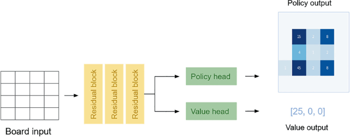
- deep neural net generates estimates for
- value of a new configuration: probability to win
- policy to explore an yet untested move
- Monte Carlo tree search uses combination of
- exploitation maximize probability to win (value)
- exploration trying out something new (policy)
- 1600 Monte Carlo tree search (MCTS) steps
→ two kinds of policies
- prior generated by deep net
- posterior generated by MCTS
- next move selected
most explored configuration
- not: configuration most likely to win!
- "supervised RL"
store entire game → error backpropagation
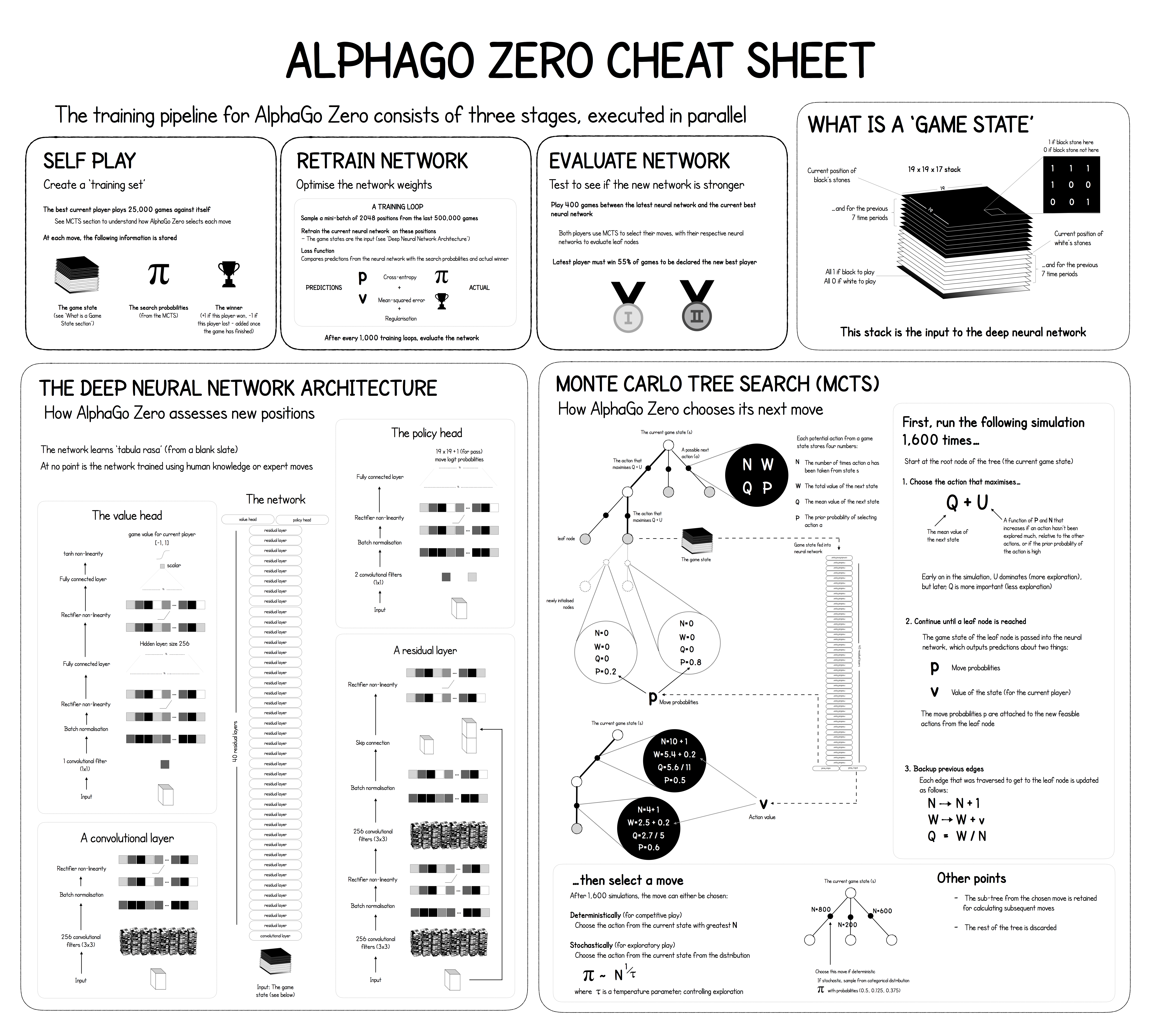
Alpha zero cheat sheet

intermezzo: neural scaling laws
scarce recourses
- compute
(total training time, in FLOPS)
- size
(total number of adjustable parameters)
- data (total amount)
(Hoffmann, et al, 2022)
- optimal parameter combination
:: empirical
compute $\ \sim\ $ (size)$^2$
- (very) large compute needed
- prefactor for small models
→ optimal scaling for production model
:: essential for large language models (LLM)
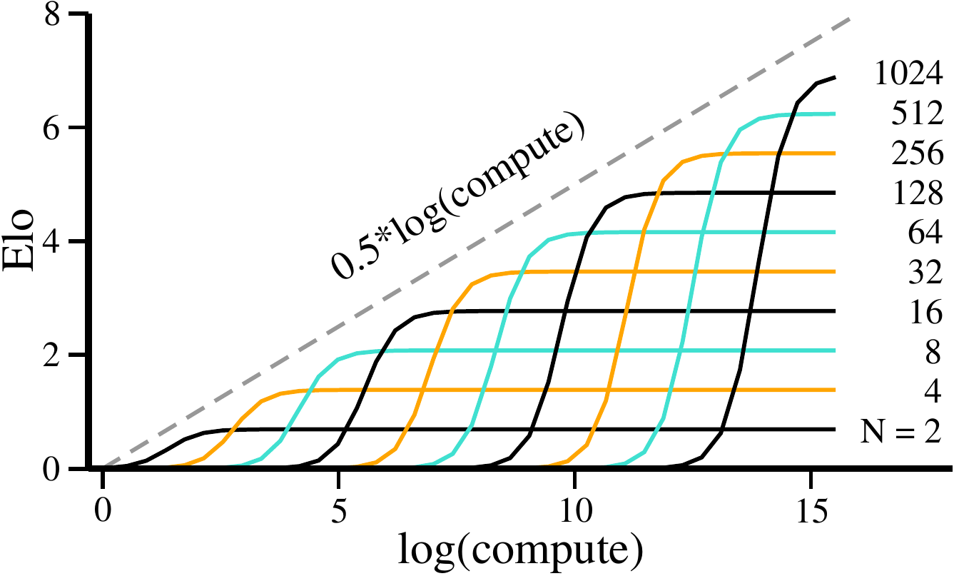
Alpha Zero Elo scaling
Elo ranking
- probability that A beats B
$\displaystyle
P(A\!\to\!B) = \frac{1}{1+10^{-(E_A-E_B)/400}}
$
societies of game playing agents
$$
P(A\!\to\!B) \approx \frac{N_A}{N_A+N_B}
$$
$$
\mathrm{Elo} \ \approx \ \log(N)\cdot\sigma\left(
\beta\log\left(\frac{\sqrt{C}}{N}\right)\right),
\quad\qquad
\mathrm{time} \propto (\mathrm{resources})^2
$$
- $\sigma()$ sigmoidal
- brain size / learning scaling?
:: brain size limitation?
