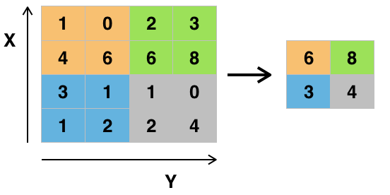
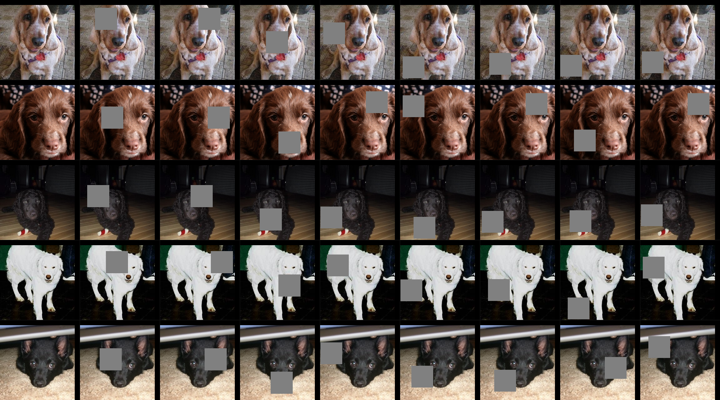
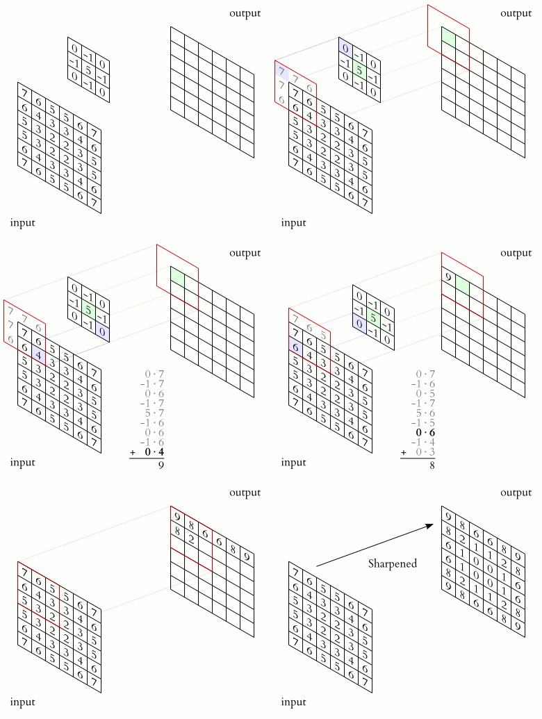
| removing | : | weak links; $|w_{ij}|$ well below average |
| reduces | : | network complexity; overfitting |
| whitening | : | covariance matrix $\to$ identity matrix |
| : | all data equally relevant |
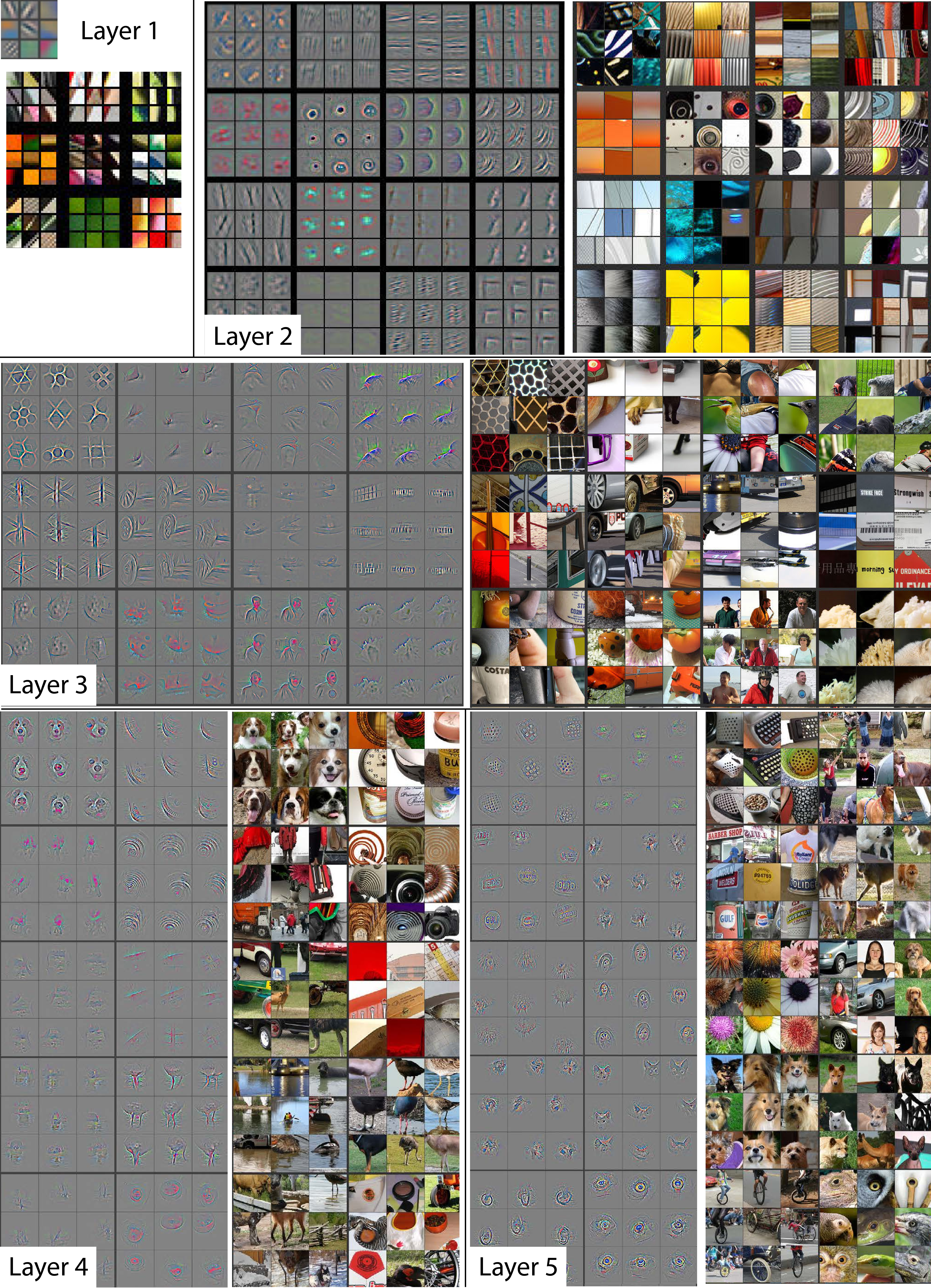
| $\to$ | hierarchical feature representation by hidden nodes |
zip() iterables → tuples
* packing, unpacking (lists, dictionaries, ..)
#!/usr/bin/env python3
# coding: utf-8
# source:
# https://www.kaggle.com/code/weka511/autoencoder-implementation-in-pytorch
from matplotlib.pyplot import close, figure, imshow, savefig, show, title
from matplotlib.lines import Line2D
from os.path import join # pathname manipulation
from random import sample # random sampling of lists
from re import split # regular expression (strings)
from torch import device, no_grad
from torch.cuda import is_available
from torch.nn import Linear, Module, MSELoss, ReLU, Sequential, Sigmoid
from torch.optim import Adam
from torch.utils.data import DataLoader
from torchvision.datasets import MNIST
from torchvision.transforms import Compose, ToTensor
from torchvision.utils import make_grid
#
# Hyperparameters
#
# 1. The sizes of the encoder layers are taken from
# [Reducing the Dimensionality of Data with Neural Networks
# G. E. Hinton and R. R. Salakhutdinov]
# (https://www.cs.toronto.edu/~hinton/science.pdf)
# 2. The learning rate was optimized by trial and error.
# The error rates are plotted here
# (https://github.com/weka511/learn/issues/26)
ENCODER = [28*28,400,200,100,50,25,6] # sizes of encoder layers
DECODER = [] # Decoder layers will be a mirror image of encoder
LR = 0.001 # Learning rate
N = 32 # Number of epochs
#
# The Autoencoder class
#
# The latest version of this class can be found at
# [github](https://github.com/weka511/learn/blob/master/ae.py)
class AutoEncoder(Module):
'''A class that implements an AutoEncoder
'''
@staticmethod
def get_non_linearity(params):
'''Determine which non linearity is to be used for both
encoder and decoder'''
def get_one(param):
'''Determine which non linearity is to be used for
either encoder or decoder'''
param = param.lower()
if param=='relu': return ReLU()
if param=='sigmoid': return Sigmoid()
return None
decoder_non_linearity = get_one(params[0])
encoder_non_linearity = \
getnl(params[a]) if len(params)>1 else decoder_non_linearity
return encoder_non_linearity, decoder_non_linearity
@staticmethod
def build_layer(sizes,
non_linearity = None):
'''Construct encoder or decoder as a Sequential of Linear
labels, with or without non-linearities
Positional arguments:
sizes List of sizes for each Linear Layer
Keyword arguments:
non_linearity Object used to introduce non-linearity between layers
'''
linears = [Linear(m,n) for m,n in zip(sizes[:-1],sizes[1:])]
if non_linearity==None:
return Sequential(*linears)
else:
return Sequential(*[item for pair in [(layer,non_linearity) \
for layer in linears] for item in pair])
def __init__(self,
encoder_sizes = [28*28,400,200,100,50,25,6],
encoder_non_linearity = ReLU(inplace=True),
decoder_sizes = [],
decoder_non_linearity = ReLU(inplace=True)):
'''Keyword arguments:
encoder_sizes List of sizes for each Linear Layer in encoder
encoder_non_linearity Non-linearity between encoder layers
decoder_sizes List of sizes for each Linear Layer in decoder
decoder_non_linearity Non-linearity between decoder layers
'''
super().__init__()
self.encoder_sizes = encoder_sizes
self.decoder_sizes = encoder_sizes[::-1] if len(decoder_sizes)==0 \
else decoder_sizes
self.encoder = AutoEncoder.build_layer(self.encoder_sizes,
non_linearity = encoder_non_linearity)
self.decoder = AutoEncoder.build_layer(self.decoder_sizes,
non_linearity = decoder_non_linearity)
self.encodeBool = True
self.decodeBool = True
def forward(self, x):
'''Propagate value through network
Computation is controlled by self.encodeBool and self.decodeBool
'''
if self.encodeBool:
x = self.encoder(x)
if self.decodeBool:
x = self.decoder(x)
return x
def n_encoded(self):
return self.encoder_sizes[-1]
#
# Function to train network
#
def train(loader, model, optimizer, criterion, N = 25, dev = 'cpu'):
'''Train network
Parameters:
loader Used to get data
model Model to be trained
optimizer Used to minimze errors
criterion Used to compute errors
Keyword parameters:
N Number of epochs
dev Device - cpu or cuda
'''
Losses = []
for epoch in range(N):
loss = 0
for batch_features, _ in loader:
batch_features = batch_features.view(-1, 784).to(dev)
optimizer.zero_grad()
outputs = model(batch_features)
train_loss = criterion(outputs, batch_features)
train_loss.backward()
optimizer.step()
loss += train_loss.item()
Losses.append(loss / len(loader))
print(f'epoch : {epoch+1}/{N}, loss = {Losses[-1]:.6f}')
return Losses
#
# Initialize network and data, and prepare to train
#
# This is proably a suboptimal way to load the MNIST dataset,
# but it will do for this example.
#
dev = device("cuda" if is_available() else "cpu")
encoder_non_linearity,decoder_non_linearity = AutoEncoder.get_non_linearity(['relu'])
model = AutoEncoder(encoder_sizes = ENCODER,
encoder_non_linearity = encoder_non_linearity,
decoder_non_linearity = decoder_non_linearity,
decoder_sizes = DECODER).to(dev)
optimizer = Adam(model.parameters(),
lr = LR)
criterion = MSELoss()
transform = Compose([ToTensor()])
train_dataset = MNIST(root="~/torch_datasets",
train = True,
transform = transform,
download = True)
test_dataset = MNIST(root="~/torch_datasets",
train = False,
transform = transform,
download = True)
train_loader = DataLoader(train_dataset,
batch_size = 128,
shuffle = True,
num_workers = 4)
test_loader = DataLoader(test_dataset,
batch_size = 32,
shuffle = False,
num_workers = 4)
#
# Train network
#
Losses = train(train_loader,model,optimizer,criterion, N = N, dev = dev)
def reconstruct(loader,model,criterion,
N = 25,
prefix = 'test',
show = False,
figs = './figs',
n_images = -1):
'''Reconstruct images from encoding
Parameters:
loader
model
Keyword Parameters:
N Number of epochs used for training (used in image title only)
prefix Prefix file names with this string
show Used to display images
figs Directory for storing images
'''
def plot(original=None,decoded=None):
'''Plot original images and decoded images'''
fig = figure(figsize=(10,10))
ax = fig.subplots(nrows=2)
ax[0].imshow(make_grid(original.view(-1,1,28,28)).permute(1, 2, 0))
ax[0].set_title('Raw images')
scaled_decoded = decoded/decoded.max()
ax[1].imshow(make_grid(scaled_decoded.view(-1,1,28,28)).permute(1, 2, 0))
ax[1].set_title(f'Reconstructed images after {N} epochs')
savefig(join(figs,f'{prefix}-comparison-{i}'))
if not show:
close (fig)
samples = [] if n_images==-1 else sample(range(len(loader)//loader.batch_size),
k = n_images)
loss = 0.0
with no_grad():
for i,(batch_features, _) in enumerate(loader):
batch_features = batch_features.view(-1, 784).to(dev)
outputs = model(batch_features)
test_loss = criterion(outputs, batch_features)
loss += test_loss.item()
if len(samples)==0 or i in samples:
plot(original=batch_features,
decoded=outputs)
return loss
#
# Compare output layer with Inputs,
# to get an idea of the quality of the encoding
#
test_loss = reconstruct(test_loader,model,criterion,
N = N,
show = True,
figs = '.',
n_images = 5,
prefix = 'foo')
def plot_losses(Losses,
lr = 0.001,
encoder = [],
decoder = [],
encoder_nonlinearity = None,
decoder_nonlinearity = None,
N = 25,
show = False,
figs = './figs',
prefix = 'ae',
test_loss = 0):
'''Plot curve of training losses'''
fig = figure(figsize=(10,10))
ax = fig.subplots()
ax.plot(Losses)
ax.set_ylim(bottom=0)
ax.set_title(f'Training Losses after {N} epochs')
ax.set_ylabel('MSELoss')
ax.text(0.95, 0.95, '\n'.join([f'lr = {lr}',
f'encoder = {encoder}',
f'decoder = {decoder}',
f'encoder nonlinearity = {encoder_nonlinearity}',
f'decoder nonlinearity = {decoder_nonlinearity}',
f'test loss = {test_loss:.3f}'
]),
transform = ax.transAxes,
fontsize = 14,
verticalalignment = 'top',
horizontalalignment = 'right',
bbox = dict(boxstyle = 'round',
facecolor = 'wheat',
alpha = 0.5))
savefig(join(figs,f'{prefix}-losses'))
if not show:
close (fig)
plot_losses(Losses,
lr = LR,
encoder = model.encoder_sizes,
decoder = model.decoder_sizes,
encoder_nonlinearity = encoder_non_linearity,
decoder_nonlinearity = decoder_non_linearity,
N = N,
show = True,
figs = '.',
prefix = 'foo',
test_loss = test_loss)
def plot_encoding(loader,model,
figs = './figs',
dev = 'cpu',
colours = [],
show = False,
prefix = 'ae'):
'''Plot the encoding layer
Since this is multi,dimensional, we will break it into 2D plots
'''
def extract_batch(batch_features, labels,index):
'''Extract xs, ys, and colours for one batch'''
batch_features = batch_features.view(-1, 784).to(dev)
encoded = model(batch_features).tolist()
return list(zip(*([encoded[k][2*index] for k in range(len(labels))],
[encoded[k][2*index+1] for k in range(len(labels))],
[colours[labels.tolist()[k]] for k in range(len(labels))])))
save_decode = model.decodeBool
model.decodeBool = False
with no_grad():
fig = figure(figsize=(10,10))
ax = fig.subplots(nrows=2,ncols=2)
for i in range(2):
for j in range(2):
if i==1 and j==1: break
index = 2*i + j
if 2*index+1 < model.n_encoded():
xs,ys,cs = tuple(zip(*[xyc for batch_features, labels in loader for xyc in extract_batch(batch_features, labels,index)]))
ax[i][j].set_title(f'{2*index}-{2*index+1}')
ax[i][j].scatter(xs,ys,c=cs,s=1)
ax[0][0].legend(handles=[Line2D([], [],
color = colours[k],
marker = 's',
ls = '',
label = f'{k}') for k in range(10)])
savefig(join(figs,f'{prefix}-encoding'))
if not show:
close (fig)
model.decode = save_decode
#
# Plot encoded data
#
# The encoding shows that the images for most digits are separated.
# It also suggest that the encoded data clouls have been made to
# live in a 5 dimensional manifold instead of needind 6.
#
plot_encoding(test_loader,model,
show = True,
colours = ['xkcd:purple',
'xkcd:green',
'xkcd:blue',
'xkcd:pink',
'xkcd:brown',
'xkcd:red',
'xkcd:magenta',
'xkcd:yellow',
'xkcd:light teal',
'xkcd:puke'],
figs = '.',
prefix = 'foo')
|
|
|
|
|
| autoencoder | restricted Boltzmann machine | recurrent network | convolution network |
| feedforward | undirected | recurrent | hierarchical feedforward |
detach()?
#!/usr/bin/env python3
#
# recurrent net performing a prediction task
#
import torch
import math
import random
import numpy as np
import matplotlib.pyplot as plt
#
# global variables
#
dimOutput = 1 # only 1 implemented
dimHidden = 40
nData = 20 # number function values
nPlot = 20 # needs to be identical!
nIter = 1000
learningRate = 4.0e-2
xMax = 3.0 # for data / plotting
Delta_T = 3 # number of time steps to predict
#
# general layer
#
class MyLayer(torch.nn.Module): # inheritance
def __init__(self, dim1, dim2): # constructor
super().__init__()
self.w = torch.zeros(dim1,dim2,requires_grad=True) # feed forward
self.v = torch.zeros(dim1,dim1,requires_grad=True) # recurrent
self.bias = torch.zeros(dim1,requires_grad=True)
self.hidden_activity = torch.zeros(dim1) # hidden activity
sigma_w = 1.0/math.sqrt(dim2)
sigma_v = 1.0/math.sqrt(dim1)
torch.nn.init.normal_(self.w, mean=0.0, std=sigma_w)
torch.nn.init.normal_(self.v, mean=0.0, std=sigma_v)
def forward(self, x): # default forward pass
yy = torch.tanh(torch.matmul(self.w,x) +
torch.matmul(self.v,self.hidden_activity)*1.0 -
self.bias)
self.hidden_activity = yy.detach() # store hidden activity
return yy
def forward_linear(self, x): # linear unit
return torch.matmul(self.w,x) - self.bias
def update_hidden(self, eps): # updating
with torch.no_grad():
self.w -= eps*self.w.grad
self.v -= eps*self.v.grad
self.bias -= eps*self.bias.grad
self.w.grad = None
self.v.grad = None
self.bias.grad = None
def update_linear(self, eps): # no recurrent connections
with torch.no_grad():
self.w -= eps*self.w.grad
self.bias -= eps*self.bias.grad
self.w.grad = None
self.bias.grad = None
#
# target: Bell curve and beyond
#
def target_curve(x):
return torch.exp(-0.5*x.pow(2)) / math.sqrt(2.0*math.pi)
# return torch.sin(x.pow(2)) + torch.cos(x)
#
# new training data, using random starting point
#
def trainingData(nPoints):
startX = -xMax + xMax*0.1*random.random()
endX = startX + 2.0*xMax
deltaX = 2.0*xMax/(nPoints-1.0)
startY = startX + Delta_T*deltaX
endY = endX + Delta_T*deltaX
#
inputPoints = torch.linspace(startX, endX, nPoints)
inputFunction = target_curve( inputPoints )
outputPoints = torch.linspace(startY ,endY, nPoints)
outputFunction = target_curve( outputPoints )
return inputPoints, inputFunction, outputPoints, outputFunction
#
# instantiate model, define forward pass
#
layerHidden = MyLayer(dimHidden,1)
layerOutput = MyLayer(dimOutput,dimHidden)
def modelForward(myInput):
hidden = layerHidden(myInput) # calling defaulf forward pass
return layerOutput.forward_linear(hidden) # linear output units
#
# training loop
#
for iIter in range(nIter): # trainning loop
inPoints, inFunction, outPoints, outFunction = trainingData(nData)
#
if iIter==-1:
for iData in range(nData):
print(inPoints[iData].item(), inFunction[iData].item())
trainingLoss = 0.0 # loss is added
for iData in range(nData): # data points == batch
# function approximation
# trainInput = inPoints[iData].unsqueeze(0) # add dimension
# trainValue = inFunction[iData]
# function prediction
trainInput = inFunction[iData].unsqueeze(0)
trainValue = outFunction[iData]
output = modelForward(trainInput) # forward pass
trainingLoss += (output-trainValue).pow(2).sum()
#
trainingLoss.backward() # backward pass
layerHidden.update_hidden(learningRate/nData)
layerOutput.update_linear(learningRate/nData)
#
tenPercent = int(nIter/10)
if (iIter%tenPercent==0):
print(f'{iIter:7d}', trainingLoss.tolist())
#
# preparing plots
#
inPoints, inFunction, outPoints, outFunction = trainingData(nPlot)
in__points_Plot = inPoints.tolist()
out_points_Plot = outPoints.tolist()
inference_Plot = [0.0 for _ in range(nPlot)]
in__F_Plot = inFunction.tolist()
out_F_Plot = outFunction.tolist()
for iPlot in range(nPlot):
# testInput = inPoints[iPlot].unsqueeze(0)
testInput = inFunction[iPlot].unsqueeze(0)
inference_Plot[iPlot] = modelForward(testInput).item()
#
# plotting
#
plt.plot(in__points_Plot, in__F_Plot, 'k', label="original curve")
plt.plot(in__points_Plot, out_F_Plot, 'g', label="shifted curve")
plt.plot(in__points_Plot,inference_Plot, '.r', label="inference", markersize=10)
plt.legend()
plt.xlabel('input activity')
plt.ylabel('output activity')
plt.savefig('foo.svg')
plt.show()
$\qquad$
|
|
|
|
#!/usr/bin/env python3
# coding: utf-8
# convolution neural net
# source:
# https://pytorch.org/tutorials/beginner/blitz/cifar10_tutorial.html
# What about data?
# ----------------
#
# Generally, when you have to deal with image, text, audio or video data,
# you can use standard python packages that load data into a numpy array.
# Then you can convert this array into a `torch.*Tensor`.
#
# Specifically for vision `torchvision` that has data loaders
# for common datasets such as ImageNet, CIFAR10,
# MNIST, etc. and data transformers for images, viz.,
# `torchvision.datasets` and `torch.utils.data.DataLoader`.
#
# The CIFAR10 dataset used here has the classes:
# 'airplane', 'automobile', 'bird', 'cat', 'deer',
# 'dog', 'frog', 'horse', 'ship', 'truck'.
#
# The images in CIFAR-10 are of size 3x32x32, i.e.
# 3-channel color images of 32x32 pixels in size.
#
#
# Training an image classifier
# ----------------------------
#
# 1. Load and normalize the CIFAR10 training and test datasets
# using `torchvision`
# 2. Define a Convolutional Neural Network
# 3. Define a loss function
# 4. Train the network on the training data
# 5. Test the network on the test data
# ### 1. Load and normalize CIFAR10
#
import torch
import torchvision
import torchvision.transforms as transforms
# The output of torchvision datasets,
# PILImage images of range [0, 1], are transformed
# to Tensors of normalized range [-1, 1].
#
transform = transforms.Compose(
[transforms.ToTensor(),
transforms.Normalize((0.5, 0.5, 0.5), (0.5, 0.5, 0.5))])
batch_size = 4
trainset = torchvision.datasets.CIFAR10(root='./data', train=True,
download=True, transform=transform)
trainloader = torch.utils.data.DataLoader(trainset, batch_size=batch_size,
shuffle=True, num_workers=2)
testset = torchvision.datasets.CIFAR10(root='./data', train=False,
download=True, transform=transform)
testloader = torch.utils.data.DataLoader(testset, batch_size=batch_size,
shuffle=False, num_workers=2)
classes = ('plane', 'car', 'bird', 'cat',
'deer', 'dog', 'frog', 'horse', 'ship', 'truck')
#
# Let us show some of the training images, for fun.
#
import matplotlib.pyplot as plt
import numpy as np
#
# function to show an image
#
def imshow(img):
img = img / 2 + 0.5 # unnormalize
npimg = img.numpy()
plt.imshow(np.transpose(npimg, (1, 2, 0)))
plt.show()
# get some random training images
dataiter = iter(trainloader)
images, labels = next(dataiter)
# show images
imshow(torchvision.utils.make_grid(images))
# print labels
print(' '.join(f'{classes[labels[j]]:5s}' for j in range(batch_size)))
# 2. Define a Convolutional Neural Network
# ========================================
#
# Copy the neural network from the Neural Networks section before and
# modify it to take 3-channel images (instead of 1-channel images as it
# was defined).
#
import torch.nn as nn
import torch.nn.functional as F
class Net(nn.Module):
def __init__(self):
super().__init__()
self.conv1 = nn.Conv2d(3, 6, 5)
self.pool = nn.MaxPool2d(2, 2)
self.conv2 = nn.Conv2d(6, 16, 5)
self.fc1 = nn.Linear(16 * 5 * 5, 120)
self.fc2 = nn.Linear(120, 84)
self.fc3 = nn.Linear(84, 10)
def forward(self, x):
x = self.pool(F.relu(self.conv1(x)))
x = self.pool(F.relu(self.conv2(x)))
x = torch.flatten(x, 1) # flatten all dimensions except batch
x = F.relu(self.fc1(x))
x = F.relu(self.fc2(x))
x = self.fc3(x)
return x
net = Net()
# 3. Define a Loss function and optimizer
# =======================================
#
# Let\'s use a Classification Cross-Entropy loss and SGD with momentum.
#
import torch.optim as optim
criterion = nn.CrossEntropyLoss()
optimizer = optim.SGD(net.parameters(), lr=0.001, momentum=0.9)
# 4. Train the network
# ====================
#
# This is when things start to get interesting. We simply have to loop
# over our data iterator, and feed the inputs to the network and optimize.
#
for epoch in range(2): # loop over the dataset multiple times
running_loss = 0.0
for i, data in enumerate(trainloader, 0):
# get the inputs; data is a list of [inputs, labels]
inputs, labels = data
# zero the parameter gradients
optimizer.zero_grad()
# forward + backward + optimize
outputs = net(inputs)
loss = criterion(outputs, labels)
loss.backward()
optimizer.step()
# print statistics
running_loss += loss.item()
if i % 2000 == 1999: # print every 2000 mini-batches
print(f'[{epoch + 1}, {i + 1:5d}] loss: {running_loss / 2000:.3f}')
running_loss = 0.0
print('Finished Training')
# Save trained model, compare
# https://pytorch.org/docs/stable/notes/serialization.html
PATH = './cifar_net.pth'
torch.save(net.state_dict(), PATH)
# 5. Test the network on the test data
# ====================================
#
# We have trained the network for 2 passes over the training dataset. But
# we need to check if the network has learnt anything at all.
#
# We will check this by predicting the class label that the neural network
# outputs, and checking it against the ground-truth. If the prediction is
# correct, we add the sample to the list of correct predictions.
#
# Okay, first step. Let us display an image from the test set to get
# familiar.
#
dataiter = iter(testloader)
images, labels = next(dataiter)
# print images
imshow(torchvision.utils.make_grid(images))
print('GroundTruth: ', ' '.join(f'{classes[labels[j]]:5s}' for j in range(4)))
# Load back saved model, for illustation,
# saving and re-loading # the model wasn't necessary.
#
net = Net()
net.load_state_dict(torch.load(PATH))
# What does the neural network thinks these examples above are?
outputs = net(images)
# The outputs are energies for the 10 classes. The higher the energy for a
# class, the more the network thinks that the image is of the particular
# class. So, let's get the index of the highest energy:
#
_, predicted = torch.max(outputs, 1)
print('Predicted: ', ' '.join(f'{classes[predicted[j]]:5s}'
for j in range(4)))
#
# Network performs on the whole dataset.
#
correct = 0
total = 0
# since we're not training, we don't need to calculate
# the gradients for our outputs
with torch.no_grad():
for data in testloader:
images, labels = data
# calculate outputs by running images through the network
outputs = net(images)
# the class with the highest energy is what we choose as prediction
_, predicted = torch.max(outputs.data, 1)
total += labels.size(0)
correct += (predicted == labels).sum().item()
print(f'Accuracy of the network on the 10000 test images: {100 * correct // total} %')
#
# Count predictions for each class.
#
correct_pred = {classname: 0 for classname in classes}
total_pred = {classname: 0 for classname in classes}
# again, no gradients needed
with torch.no_grad():
for data in testloader:
images, labels = data
outputs = net(images)
_, predictions = torch.max(outputs, 1)
# collect the correct predictions for each class
for label, prediction in zip(labels, predictions):
if label == prediction:
correct_pred[classes[label]] += 1
total_pred[classes[label]] += 1
# print accuracy for each class
for classname, correct_count in correct_pred.items():
accuracy = 100 * float(correct_count) / total_pred[classname]
print(f'Accuracy for class: {classname:5s} is {accuracy:.1f} %')
# Assuming that we are on a CUDA machine, this should print a CUDA device:
device = torch.device('cuda:0' if torch.cuda.is_available() else 'cpu')
print(device)
del dataiter