Machine Learning Primer -- Basics


Claudius Gros, WS 2024/25

Institut für theoretische Physik
Goethe-University Frankfurt a.M.

Information Theory

probability distributions


examples

power laws

normalized probability distribution functions
may have a diverging mean and/or variance
Copy Copy to clipboad
Downlaod Download
#!/usr/bin/env python3
# plotting a few distribution functions

import math                      # math
import numpy as np               # numerics
import matplotlib.pyplot as plt  # plotting

max_X   = 5.0
nPoints = 100

xData   = [ii*max_X/nPoints for ii in range(nPoints)]

yNormal = [math.exp(-0.5*xx*xx) for xx in xData]
yExp    = [math.exp(-xx)        for xx in xData]
yTsalis = [1.0/(1.0+xx)**2      for xx in xData]

plt.plot(xData, yNormal, "ob", markersize=4, label="normall")
plt.plot(xData, yExp,    "og", markersize=4, label="exponential")
plt.plot(xData, yTsalis, "or", markersize=4, label="Tsalis-Pareto")
#
plt.xlim(0, max_X)
plt.ylim(0, 1.05)                 # axis limits
plt.legend(loc="upper right")     # legend location
plt.savefig('foo.svg')            # export figure
plt.show()

central limit theorem
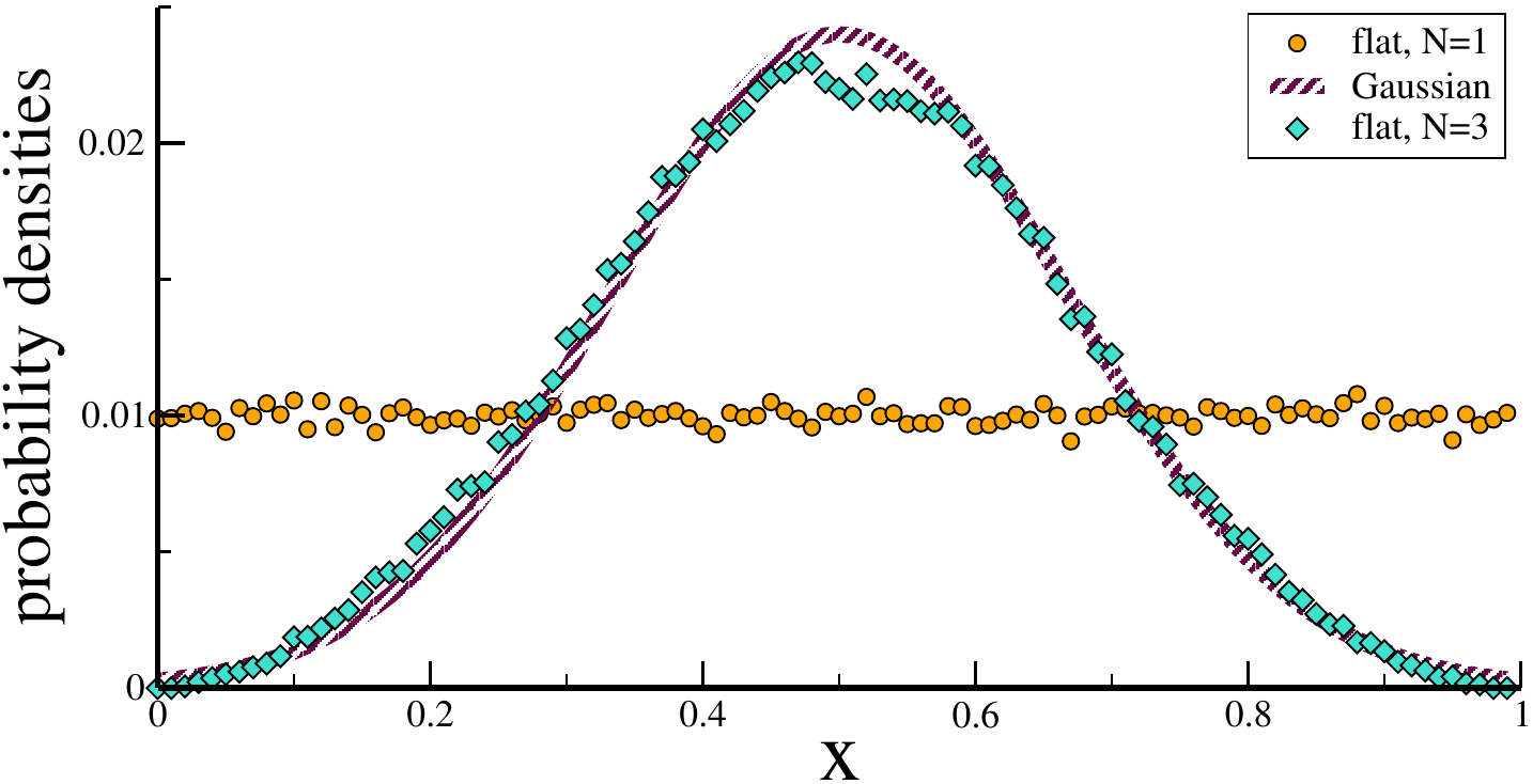


the probability distribution of a
sum of statistically independent
stochastic variables
converges to a Gaussian


law of large numbers

the variance of a
sum of statistically independent
stochastic variables
is additative


Copy Copy to clipboad
Downlaod Download
#!/usr/bin/env python3

# sum of uniform distributions, binning with 
# np.histogram()

import numpy as np               # numerics
import matplotlib.pyplot as plt  # plotting

nData = 10000
nBins = 20

# ploting at bin midpoints
xData = [(iBin+0.5)/nBins for iBin in range(nBins)]

# (adding) uniform distributions in [0,1]
data_1 = [ np.random.uniform()      for _ in range(nData)]
data_2 = [(np.random.uniform()+\
           np.random.uniform())/2.0 for _ in range(nData)]
data_3 = [(np.random.uniform()+\
           np.random.uniform()+\
           np.random.uniform())/3.0 for _ in range(nData)]

hist_1, bins = np.histogram(data_1, bins=nBins, range=(0.0,1.0))
hist_2, bins = np.histogram(data_2, bins=nBins, range=(0.0,1.0))
hist_3, bins = np.histogram(data_3, bins=nBins, range=(0.0,1.0))
#print("Bin Edges", bins)
#print("Histogram Counts", hist_1)

y_one   = hist_1*nBins*1.0/nData      # normalize
y_two   = hist_2*nBins*1.0/nData    
y_three = hist_3*nBins*1.0/nData    

plt.plot(xData, y_one,   "ob", markersize=4, label="flat-one")
plt.plot(xData, y_two,   "og", markersize=4, label="flat-two")
plt.plot(xData, y_three, "or", markersize=4, label="flat-three")
plt.plot(xData, y_three,  "r")
#
plt.xlim(0, 1)
plt.ylim(0, 2.5)
plt.legend(loc="upper right")    
plt.savefig('foo.svg')          
plt.show()
conditional probability

Bayes theorem

$$ p(x,y) = p(x|y) p(y) = p(y|x) p(x) \quad\qquad \fbox{$\phantom{\big|} p(y|x) = \frac{p(x|y) p(y)}{p(x)} \phantom{\big|}$} $$

Bayesian inference

$$ \fbox{$\phantom{\big|} p(y|x) = \frac{p(x|y) p(y)}{p(x)} \phantom{\big|}$} $$
$$ \left(\begin{array}{c} \mathbf{prior} \\ p(y) \end{array}\right) \ \longrightarrow\ \left(\begin{array}{c} \mathbf{data} \\ x \end{array}\right) \ \longrightarrow\ \left|\begin{array}{c} \mathrm{Bayes} \\ \mathrm{theorem} \end{array}\right| \ \longrightarrow\ \left(\begin{array}{c} \mathbf{postior} \\ p(y|x) \end{array}\right) \ \longrightarrow\ \left|\begin{array}{c} \mathrm{new} \\ \mathrm{prior} \end{array}\right| $$

Baysian coin flips

Copy Copy to clipboad
Downlaod Download
#!/usr/bin/env python3

import numpy as np

# ***
# *** global variables
# ***
trueBias = 0.3                             # true coin bias
nX       = 11                              # numerical discretization
xx = [i*1.0/(nX-1.0) for i in range(nX)]   
pp = [1.0/nX  for _ in range(nX)]          # starting prior

# ***
# *** Baysian updating
# ***
def updatePrior():
  """Bayesian inference for coin flips;
     marginal correspond to normalization of posterior"""
#
  evidence = 0.0 if (np.random.uniform()>trueBias) else 1.0   # coin flip
  for iX in range(nX):     
    prior = pp[iX]
    likelihood = xx[iX] if (evidence==1) else 1.0-xx[iX]
    pp[iX] = likelihood*prior              # Bayes theorem
#
  norm = sum(pp)
  for iX in range(nX):                     # normalization of posterior
    pp[iX] = pp[iX]/norm
#
  return evidence
    
# ***
# *** main
# ***

ee = 0.0
for _ in range(200):                      # iteration over observations
  for iX in range(nX):     
    print(f'{pp[iX]:6.3f}', end="")
  print(f' | {ee:3.1f}')
  ee = updatePrior()                     
#
for iX in range(nX):                      # support points
  print(f'{xx[iX]:4.1f}  ', end="")
print()

Baysian statistics

case study


maximum likelihood

maximize probability to
observe a given event
$\qquad\qquad\fbox{$\displaystyle \ \ \frac{\partial}{\partial\vartheta}\,\mathcal{L}(\vartheta|x) = 0\ \ $}$

log likelihood

batch / online processing


entropy

$$ \mathrm{high\ entropy}\ \hat{=}\ \left\{ \begin{array}{rcl} \mathrm{large\ disorder} & & \mathrm{physics}\\[0.1ex] \mathrm{high\ information\ content} &\phantom{s}& \mathrm{information\ theory}\\ \end{array} \right. $$

extensive information

Shannon entropy

$$ \fbox{$\displaystyle\ \ H[p] = -\sum\nolimits_{x_i} p(x_i)\,\log_b(p(x_i)) = -\langle\,\log_b(p)\,\rangle \ \ $} \qquad\quad H[p] \ge 0 $$

Shannon source coding theorem

Given a random variable $x$ with a PDF $p(x)$ and entropy $H[p]$.

For $N\to\infty$, the cumulative entropy $N H[p]$ is a lower bound
for the number of bits necessary for the lossless compression
of $N$ independent processes drawn from $p(x)$.

example


maximal entropy distributions

maximal entropy distributions

$$ H[p] = -\sum_{\alpha=1}^M p_\alpha\log(p_\alpha) = -\frac{M}{M}\log(1/M) = \log(M),\qquad\quad p_\alpha = \frac{1}{M} $$

entropy in physics

statistical physics

$$ H[p]=-k_BT\big\langle \ln(p)\big\rangle, \qquad\quad \beta=\frac{1}{k_bT} $$ $$ \begin{array}{rcl} \mbox{micro-canonical ensemble} && \mbox{minimal entropy} \\[1ex] \mbox{canonical ensemble} && \mbox{minimal entropy, given an energy E} \\ && \mbox{Boltzman distribution} \ \ \fbox{$\phantom{\big|} p_\alpha\sim\exp(-\beta E_\alpha) \phantom{\big|}$} \\[1ex] \mbox{grand-canonical ensemble} && \mbox{minimal entropy, given energy E, particle number N} \\ && \mbox{Boltzman distribution} \ \ \fbox{$\phantom{\big|} p_\alpha\sim\exp(-\beta (E_\alpha-\mu N)) \phantom{\big|}$} \\ \end{array} $$

entropy as a measure of disorder

$$ H(T)\quad\to\quad \left\{\begin{array}{rcl} 0 &\mbox{for}& T\to0 \\[1ex] Nk_B\ln(f) &\mbox{for}& T\to\infty \end{array}\right. $$

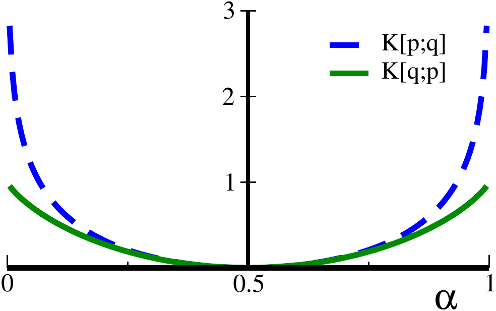
Kullback-Leibler divergence

$\displaystyle K[p;q] = \int p(x)\log\left(\frac{p(x)}{q(x)}\right)dx$

example

$$ p(0) = 1/2 = p(1) \quad\quad q(0) = \alpha\quad\quad q(1) = 1-\alpha $$

cross-entropy loss

$$ K[\mathbf{P}_t;\mathbf{P}] = \sum_i P_{t,i}\log\left( {P_{t,i}\over P_i}\right) = \sum_i P_{t,i}\log\left( P_{t,i}\right) - \sum_i P_{t,i}\log\left(P_i\right) $$

cross entropy loss

$\displaystyle L = -\sum\nolimits_i P_{t,i}\log\left(P_i\right) $