Advanced Introduction to C++, Scientific Computing and Machine Learning


Claudius Gros, SS 2024

Institut for Theoretical Physics
Goethe-University Frankfurt a.M.

Deep Learning

simple vs. complex problems


simple problems

backpropagation fails for simple problems

complex problems

given enough (labeled) training data, large
classes of complex problems are 'solvable'

deep networks


pruning
removing : weak links;
$|w_{ij}|$ well below average
reduces : network complexity;
overfitting


data preprocessing
whitening : covariance matrix
$\to$ identity matrix
: all data equally relevant

batch learning

'online' learning

offline learning

deep belief nets (DBN)


stacked RBMs

data availability

semi-supervised learning

train a net of stacked RBMs with unlabelled data
add a final output node connected to top hidden layer
use backpropagation on labelled data
to fine-tune connection weights

autoencoder


dimensionality reduction

autoencoders generate low-dimensional
representations of the (raw) data;
in the 'latent space'

denoising

stacked autoencoders

deep learning building blocks


autoencoder restricted Boltzmann machine recurrent network convolution network
feedforward undirected recurrent hierarchical feedforward

backpropagation through time

$$ \fbox{$\phantom{\big|} \mathbf{y}(t+1) \phantom{\big|}$} \quad\leftarrow\quad \fbox{$\phantom{\big|} \mathbf{y}(t) \phantom{\big|}$} \quad\leftarrow\quad \fbox{$\phantom{\big|} \mathbf{y}(t-1) \phantom{\big|}$} \quad\leftarrow\quad \fbox{$\phantom{\big|} \mathbf{y}(t-2) \phantom{\big|}$} \quad\leftarrow\quad\dots $$

receptive fields as convolutions


receptive fields

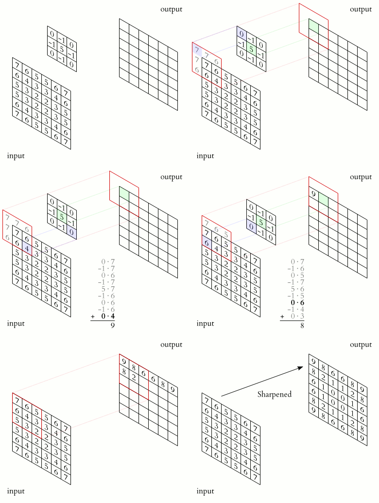
convolution scanning of 2D data


convolution networks

convolution nets

extended set of kernels
$\qquad\Rightarrow\qquad$
rastering
$\qquad\Rightarrow\qquad$
data convolution

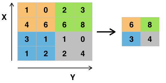
pooling

$\qquad$
  • convolution $\ \to \ $ feature map
  • pooling
    : subsampling
    : dimensionality reduction
    : e.g. max-pooling

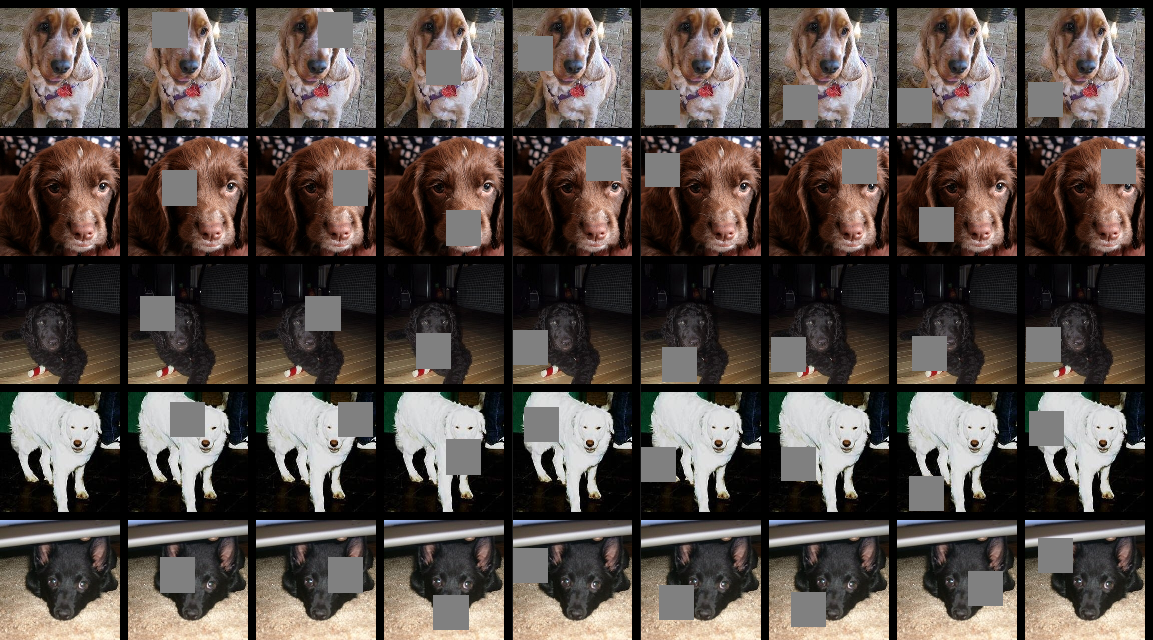
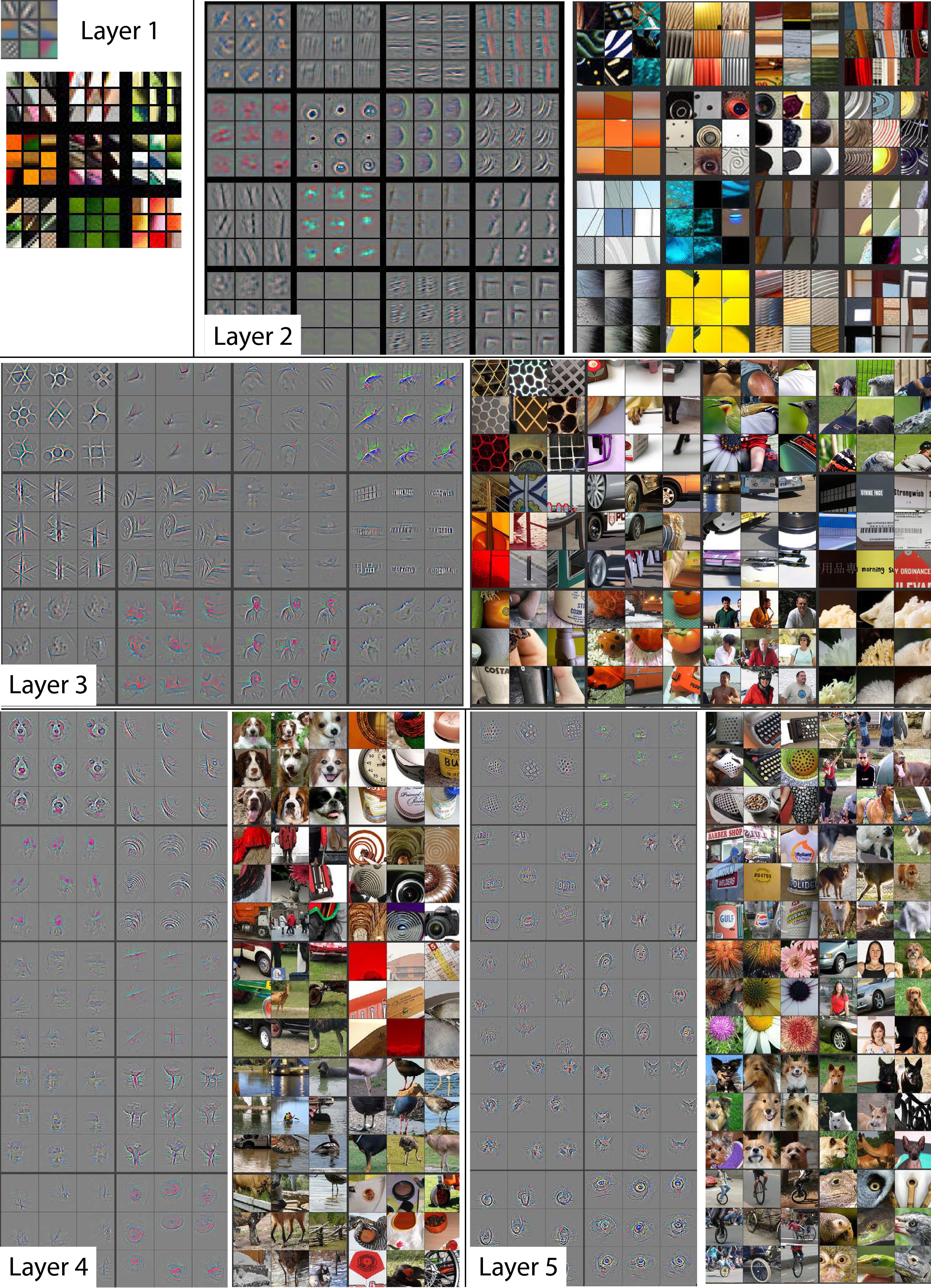
what makes it work


convolution net - illustration


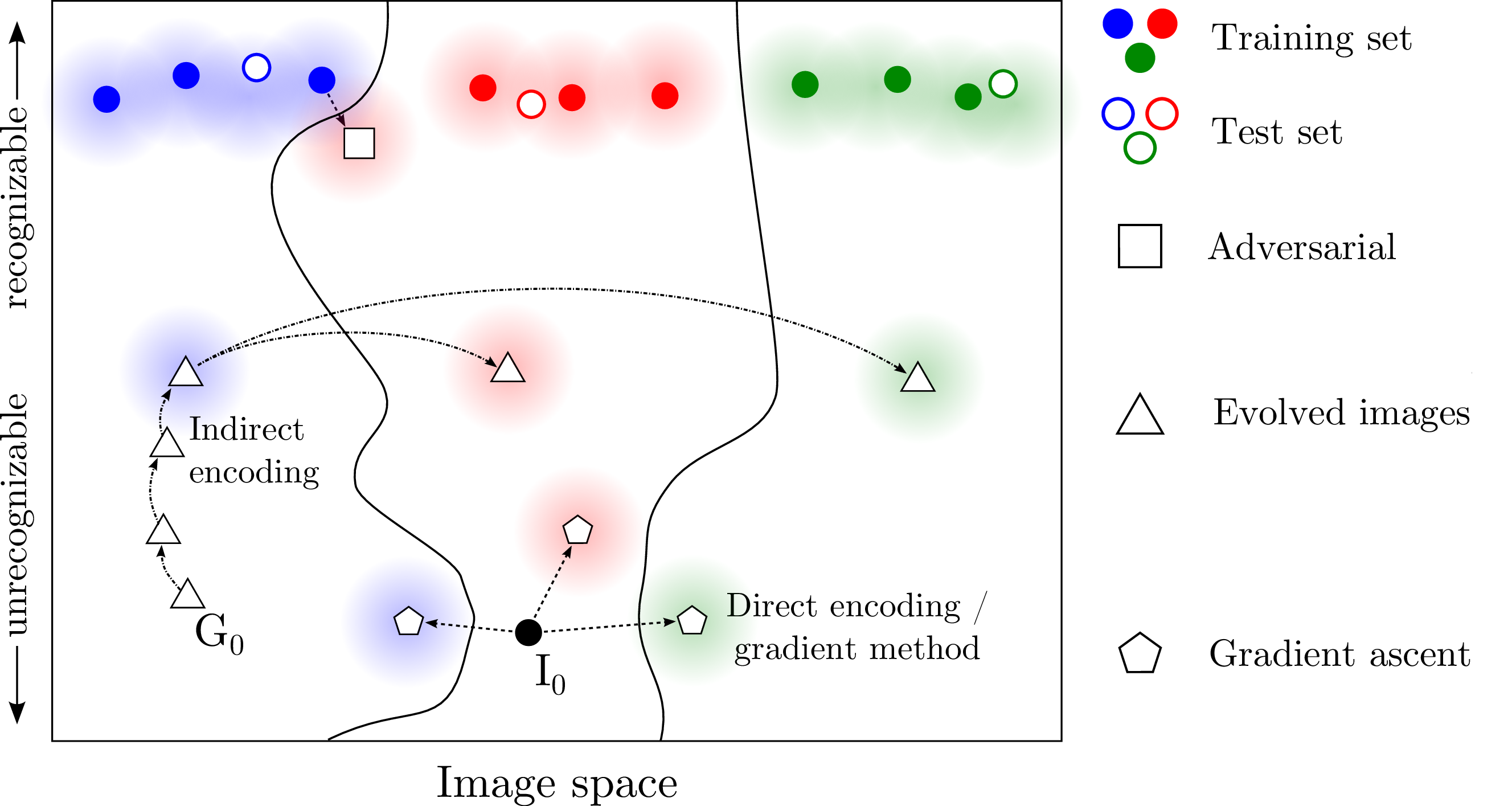
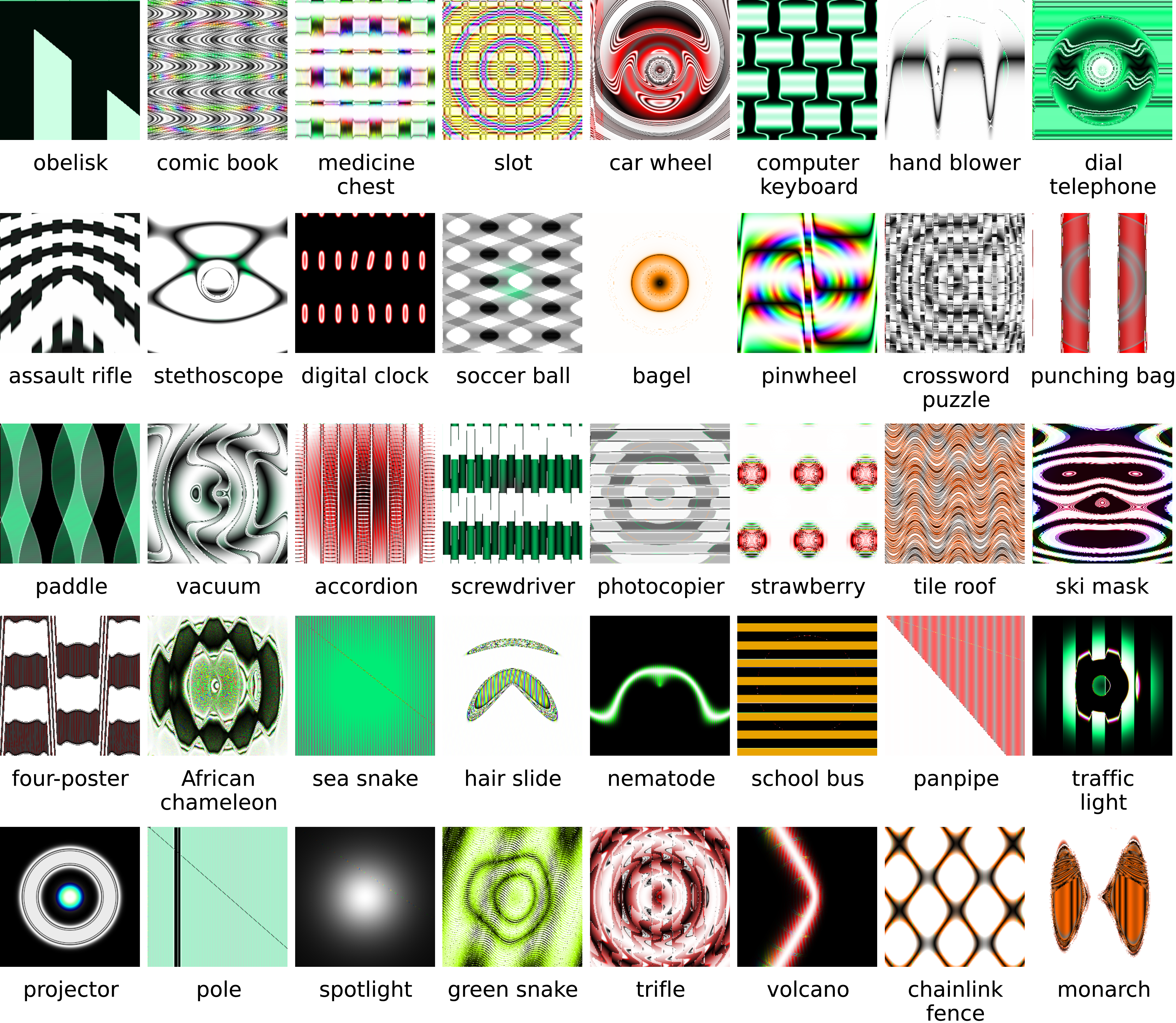
fooling deep networks


adversial perturbations


+ 0.007 x =
"panda" "nematode" "gibbon"
57.7% confidence 8.2% confidence 99.3 % confidence

performance / confidence

attacking deep networks


original tempered

cyber security

image datasets

temper train data

missclassification induced by training data tempering

$$ \begin{array}{lcccc} \hline & \rlap{\text{baseline}} & & \rlap{\text{tampered}} \\ & \text{CIFAR} & \text{SVHN} & \text{CIFAR} & \text{SVHN} \\ \hline \text{optimal case} & 0 & 0 & 100 & 100 \\ \hline \text{BCNN} & 28.7 & 12.9 & 87.2 & 91.4 \\ \text{AlexNet} & 11.1 & 5.5 & 83.7 & 97 \\ \text{VGG-16} & 5.3 & 3.7 & 90.1 & 98.9 \\ \text{ResNet-18} & 23.8 & 3.6 & 42.4 & 40.9 \\ \text{SIRRN} & 4.7 & 3.9 & 74.1 & 89.5 \\ \text{DenseNet-121} & 2.6 & 2.6 & 60.7 & 68.1 \\ \hline \end{array} $$

PyTorch

Copy Copy to clipboad
Downlaod Download
#!/usr/bin/env python3

import torch                     # PyTorch needs to be installed

dim = 2
eps = 0.1
x = torch.ones(dim, requires_grad=True)  # leaf of computational graph
print("x      : ",x)
print("x      : ",x.data)

y = x + 2
out = torch.dot(y,y)             # scalar product
print("y      : ",y)
print("out    : ",out)
print()

out.backward()                   # backward pass --> gradients
print("x.grad : ",x.grad)

with torch.no_grad():            # detach from computational graph
  x -= eps*x.grad                # updating parameter tensor 
  x.grad = None                  # flush

print("x      : ",x.data)
torch.dot(x+2,x+2).backward()
print("x.grad : ",x.grad)

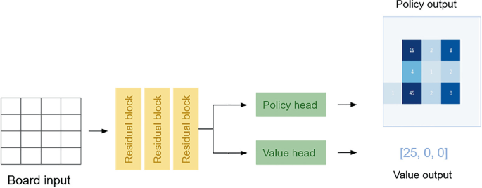
AlphaGo zero


game of Go

most explored configuration

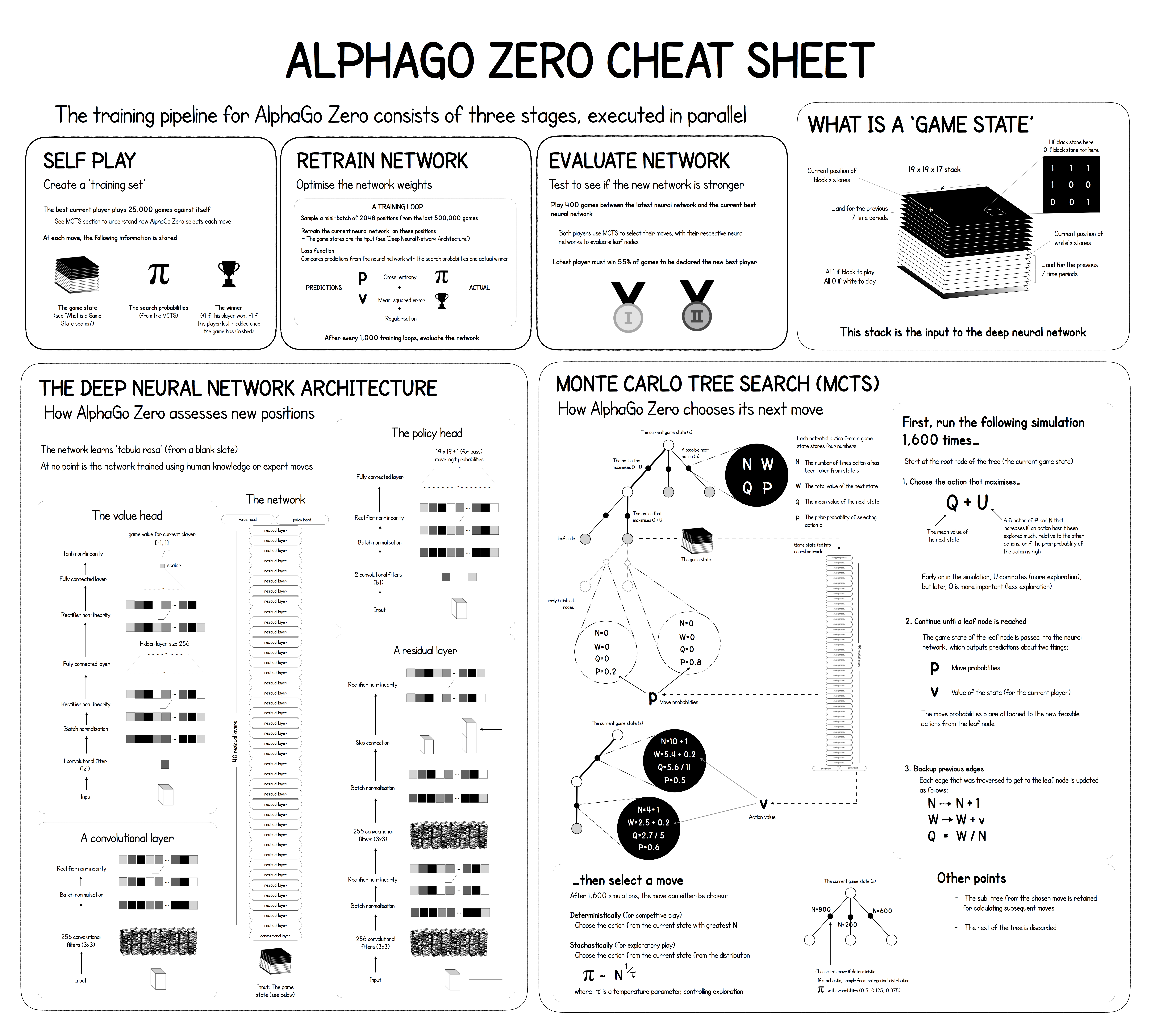
Alphago zero cheat sheet