Reinforcement learning with SARSA

SARSA (State-Action-Reward-State-Action) is a Q-learning algorithm where an agent learns to find his goal through a specific reward system.

Q-Learning is a type of problem solving where the system is being reinforced through specific decision making and reward functions. The goal is long-term and once it has reached its peak efficiency, there are barely any observable changes.

A certain quality function Q helps the agent predict the value of an action a to take in each of the states s to find its goal most efficiently. That function in turn is then updated after every action taken by the agent depending on the reward r the agent receives.

The quality function Q can be described by the Bellman equation:

Q(s_t,a_t) = Q(s_t,a_t) + ɑ[r_t+1 + ɣ Q(s_t+1,a_t+1)-Q(s_t,a_t)]

The Bellman equation named after Richard E. Bellman can be used for certain optimization problems in dynamical programming. In principle the Bellman equation describes a function which connects the value of a decision with it's possible payoff, where ɑ describes the learning rate and ɣ describes the discount factor which adjusts the impact of the actions possible after a step. It has to be < 1.

Actions are taken according to the ε-greedy policy in which the agent takes a random step in ε cases and otherwise picks the highest value action. It is common to pick ε = 0.1

To begin with the agents environment is simple. It recieves a negative reward for each step of -1 and lastly a reward of 100 for reaching the goal. The next difficulty level includes a cliff where the agent recieves a negative reward of -100 for falling off a cliff. Lastly the agent is additionally exposed to a windy environment. The wind drags the agent towards a cliff drop also added to the environment. For each new column the intensity of the wind changes, having been generated randomly at the start of the simulation.

To highlight the learning capacity of the agent the simulation shows the trajectory and movement for each episode.

The following videos and images show different ideal paths for the agent regarding certain changes of the control parameters in the Bellman equation and the grid world environments.

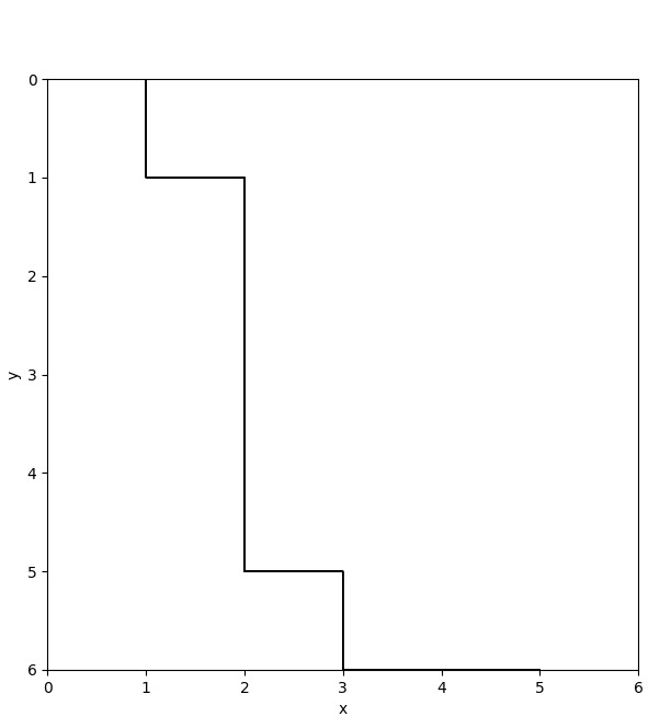
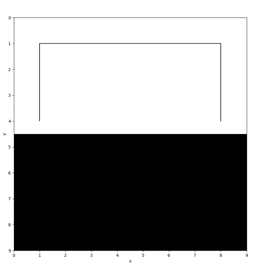
The first image shows the agent's ideal path after 100 episodes, where ɑ and ɣ equal 0.5:

With the following trajectories:

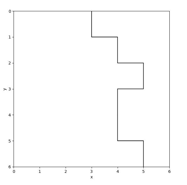
Now ɑ and ɣ equal 0.9:

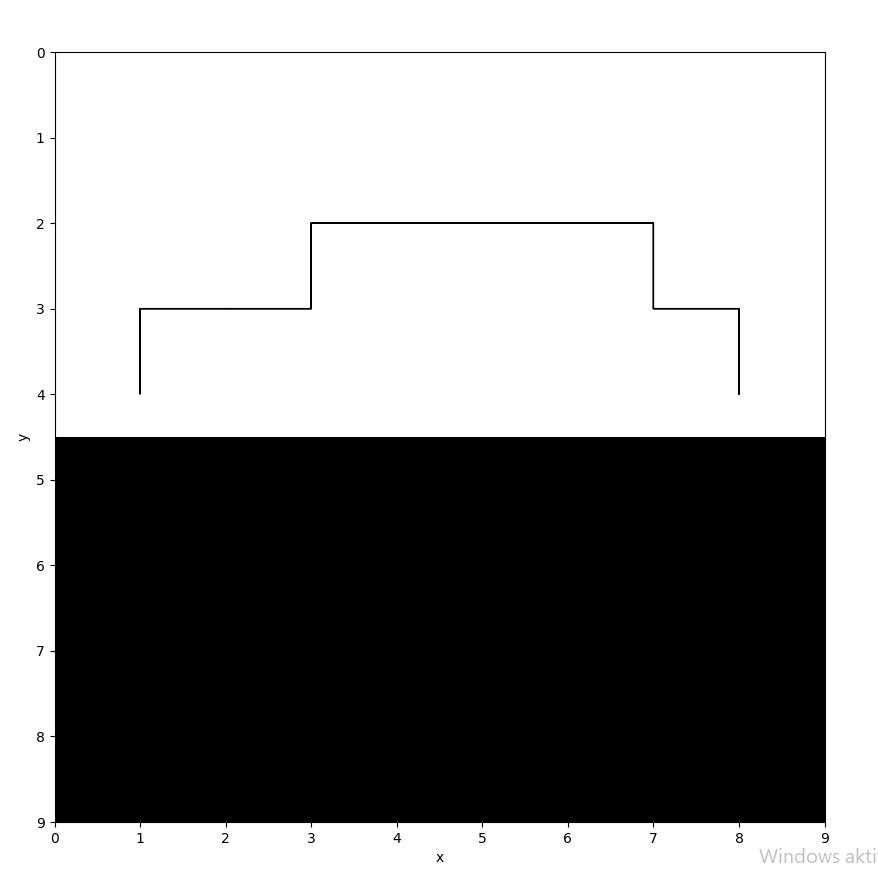
Next, the difficulty slightly increases by adding the cliff into the grid-world. The subsequent images show different ideal paths for ɑ and ɣ equaling 0.5 but this time for varying ε-values.

For ε = 0.1:

With the following trajectories taken by the agent for ε = 0.1:

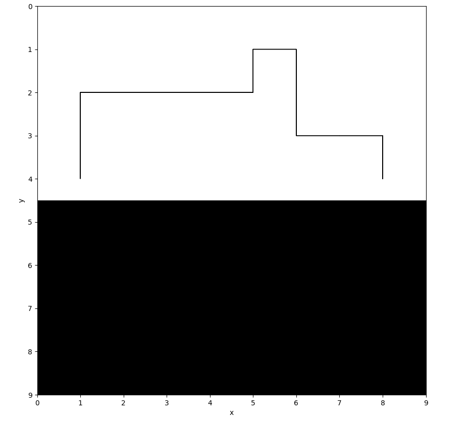
For ε = 0.2:

And lastly for ε = 0.3, where the agent went through 10000 episodes to find the ideal path:

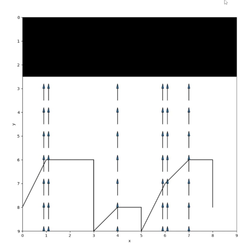
The final image shows the agents ideal path in the windy environment with a cliff drop added to it, for ε = 0.1 and ɑ and ɣ equaling 0.5:

And again, subsequently showing the paths taken by the agent: