Train of 2-wheeled cars
by Andreas Barthen and Maximilian Märcz
Introduction
In nature there are several instances in which seemingly unorganized groups of oscillators randomly start to synchronize. For example the chirping of crickets, the flashing of fireflies or even more interesting cell in the human body, like network pacemaker cells in the heart or circadian pacemaker cells in the suprachiasmatic nucleus of the brain. To get a deeper understanding of the problem we were tasked to simulate a situation in which spontaneous synchronization might occur.
Our task
Build a train of cars connecting two-wheeled cars through passive joints or springs. Implement simple a simple sinusoidal control signal separately for each car and investigate whether synchronization is possible.
The Robot
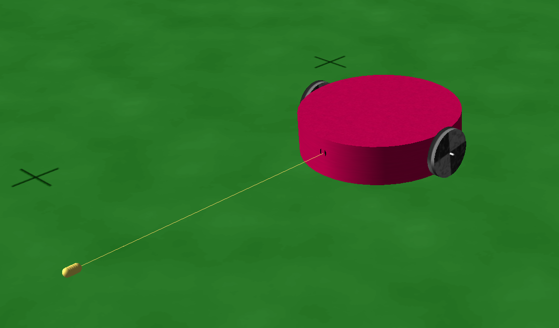
FIG. 1.a: 1 2-wheeld car with spring
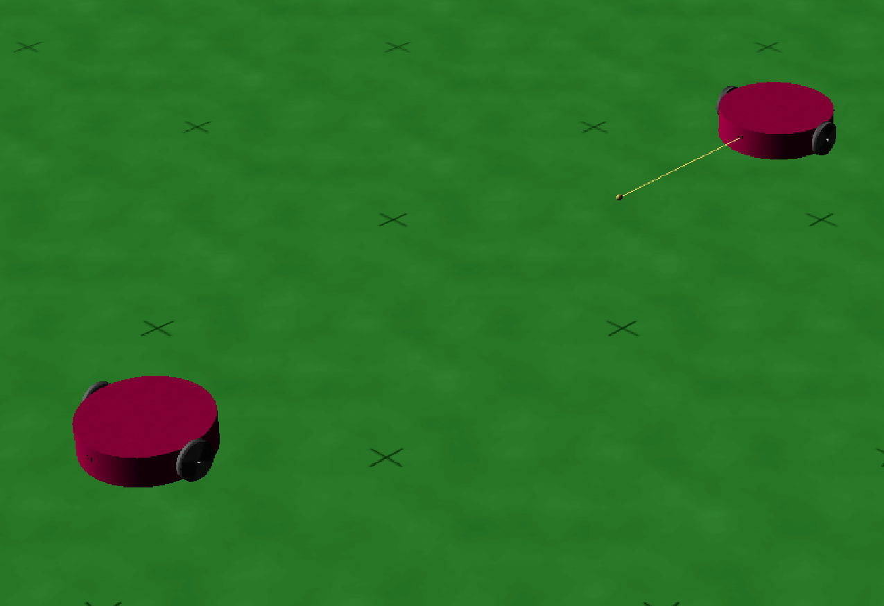
FIG. 1.b: 1 2-wheeld car with spring
As you can see in FIG. 1.a, our robot is basically the differential-robot. We used its code, removed the IR-sensors and added a spring for
distance regulation.
In FIG. 1.b you can see that one end of the spring is attached in the middle of the car and the other end is allways a fixed lenght behind the car in front.

FIG. 2: basiccontroller
Every robot was supposed to have a simple sinusoidal control signal so we added a variable called "zeit" in the basiccontroller (FIG. 2) and every simulation step, we added a constant number to it. After that we used "zeit" to calculate the speed of the robot with a simple sin function. To make sure that the robots do not all start with the same phase we added a random phase during initialization of the controller.
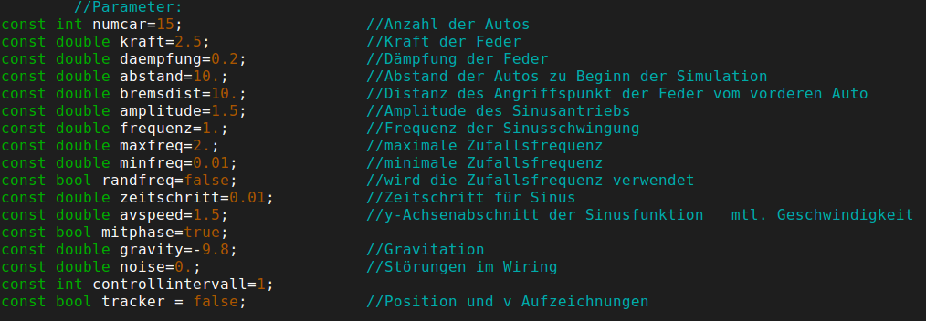
FIG. 3: setable parameters of the simulation
To be able to simply modifying the simulation, we added a lot of global parameters (FIG. 3) which can be set in the "main.cpp". Here you can set the amplitude, frequency, y-translation (averagespeed) and whether there is a random phase and frequency or not. There are also parameters for the spring and some others for the simulation e.g. the amount of cars in the train.

FIG. 4:Operator simulating the spring
In the main.cpp we added the "PulltoPointOperator" (FIG. 4) which we use as the spring. With this operator we can change the position, force, the dimensions in which the force is active, a minimum distance and the damping. The position we set to be pulled towards, is a set length behind the car right in front of it. We implemented it this way, because there should be a minimum distance between the cars and also it can be compared to the relaxation distance of a spring. If a car comes closer than that distance to the next car the spring has to force it back to the set distance, therefore slowing it down. If the distance to the car in front of it is larger than the set distance, the spring will pull the car towards the set distance, therefore speeding it up.

FIG. 5: refreshing the position of the spring
In every step of the simulation we have to set the position of the spring of each car to the new optimum position behind the car in front of it. (FIG. 5)
Videos
VID. 1: synchronization of phase between few robots
VID. 2: large springconstant
Result
Our goal was to find out whether synchronization of multiple cars is possible or not.
To check if it is possible we tracked the position and velocities of all robots in the train. Our problem was one dimensional, as if the cars were on train tracks. This is why our data is also limited to one dimension.
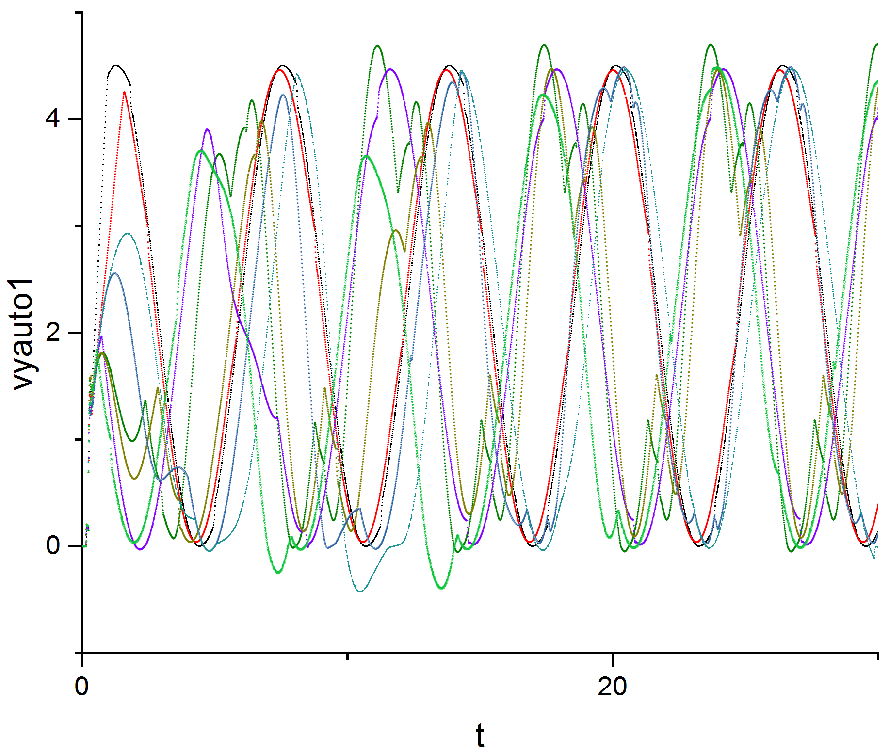
FIG. 6: velocitys of the cars
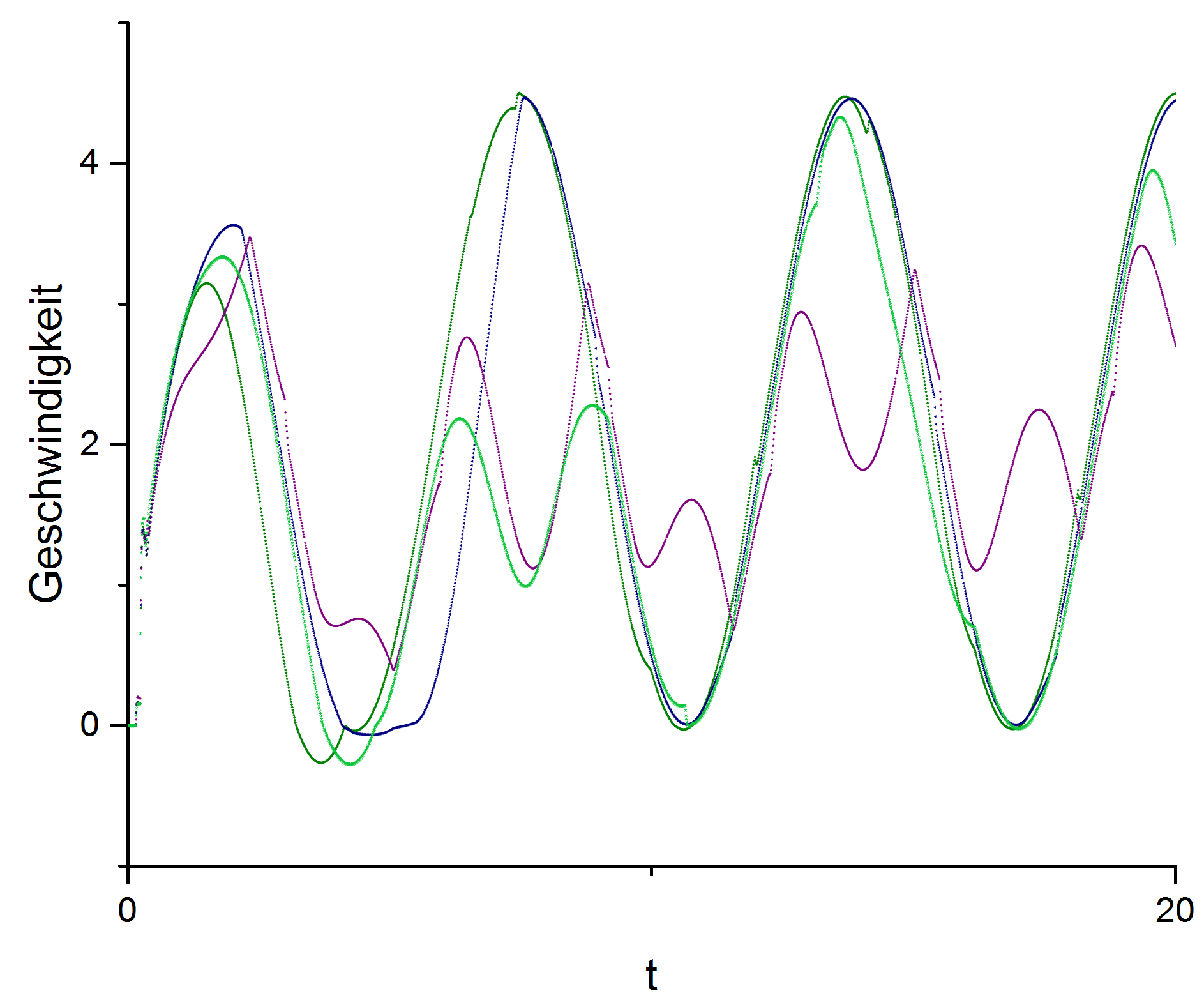
FIG. 7: velocitys of the cars with different parameters and less cars
FIG. 6 and FIG. 7 show the velocity of the cars mapped to the time of the simulation. We discarded the information about the cars, that did not synchronize with any other car to clean up the graphics. Looking at FIG. 6 one can spot the process of synchronization. You can see it best, if you work backwards. At the right side of the graphic (t>20) one can make out two groups of synchronized cars. The purple and green group and the red and blue group. Looking back at the start of the simulation (t<10) one can see, that those two groups, did not start with the level of synchronization as seen in the later time steps. FIG. 7 shows another simulation in which less cars synchronized.
It is interesting to see, that the synchronization happens really quick. In only one time period the cars are mostly synchronized and stay that way untill the end of the simulation.
As can be seen in our videos, we had some problems with the cars staying on the one dimensional track. This might be solved by actually implementing a physical 'train track' which forces the cars to stay in their one dimensional movement.
By using a very high force setting for our spring, we were able to achieve almost perfect synchronization (VID. 2), but that was obviously going to happen, thereby making that result not very satisifying. The sheer amout of parameters and the limited time prohibited us from finding other settings, which would not brute force the cars into synchronization but achieve synchronization after a short time period, as seen in FIG. 6 & 7 but with more or even all cars.
All in all we were satisfied with our results, although they might not have been as perfect as desired, because it took us a long time to actually figure out how to implement a spring into this simulation. With our code, some time and the desire to do so, it would be possible to recreat and optimize our simulations, to be able to get more accurate results.
You can download our full code here:
For our project we used the simulation program LPZ-Robots from the university of Leipzig.
This is their website: LPZ-Robots
We want to thank our tutors Laura Martin, Bulcsú Sándor and Hendrik Wernecke for supporting us with the code during the project.
To get an overview over the theory behind this problem we read:
- Strogatz S (2000). From Kuramoto to Crawford: Exploring the onset of synchronization in populations of coupled oscillators. Physica D 143 (1-4): 1-20. http://www.sciencedirect.com/science/article/pii/S0167278900000944