

Modern traffic research is going to be more an more complex due to the growing number of road users and the resulting increase of traffic density. Therefore, there is a high demand to find solutions to prevent traffic jam. There are, of course, circumstances like roadworks and traffic accidents that hinder a linear traffic flow, but there are preventable circumstances for example the "snowball effect" where a small driving error enforces and can cause a traffic jam. Future concepts are focusing on self-controlled cars with the ability to avoid traffic jams, so that the density of cars can get maximal.
Consider the following situation: we are driving on a single-lane road with all cars moving at the same velocity and distance. Suddenly, the driver in front reduces his speed. This causes us to reduce our speed as well or precisely even more because of our reaction time. It is likely that we will not reestablish our original distance but will enlarge the distance even more which forces the car behind us to slow down as well. This is a probable scenario of driving errors propagating through a line of cars.
In physics we describe observed phenomena by mathematical equations. A common way of solving a problem is to take a well known model with comparable behaviour and adapt it to the problem at hand. In our case we can describe the reaction to the car in our front with a damped oscillation around a "comfort distance". The spring rate will 'measure' the reaction time and the damping constant will determine how well the driver can estimate and adapt to the situation.
The differential equation for the damped harmonic oscillator can be written as:
$$ \begin{array}{rcl} \dfrac{dv}{dt} = \kappa (d-d_0) - \gamma \cdot v(t) \end{array} $$
with spring rate $\kappa$, damping constant $\gamma$ and the rest position $d_0$. mass $m$ = 1.
Furthermore we add a maximal and a minimal velocity to the oscillator model. Because of a technical limit and speed restrictions a maximal speed is a reasonable limitation and a minimal speed is also a realistic assumption for a driver is not likely to drive arbitrarily slow but will rather stop if he can not go faster than e.g. walking speed. In addition to that we introduced a small distance we call "crash distance" which leads to a full stop of the car to prevent crashes.
LPZ Robots allows us to set the velocity of a car in every simulation step. To implement the equation, we used the explicit Euler method to calculate the velocity for the next timestep.
$$ \begin{array}{rcl} v(t+dt) &=& v(t) + \dot{v}(t)dt \\ v(t+dt) &=& v(t) + \left[ \kappa (d-d_0) - \gamma \cdot v(t) \right] dt \end{array} $$
The basis of our simulation is the two wheeled robot which is introduced as basic example in the LPZ Robots package. The distance of the robot in front is measured by Infrared (IR) sensors. The IR sensor signal decreases with the distance of an obstacle in front in a linear fashion: distance = sensor range * (1 - sensor value). Moreover we had to attach a third wheel to the robot to prevent it from tilting and touching the floor upon accelerating.
We implemented two controllers: the basic controller which contains the driving model as described above and a leading controller to control the first robot of the queue seperatly.
The following parameters establish our standard parameter set we used for the simulation. To analyze the behaviour we changed one of parameter and left all other parameters constant.
| $\kappa = 0.25$ | The spring rate combines reaction time and strength of accelaration. |
| $\gamma < 2 \sqrt{\kappa}$ | We want to have the underdamped case of oscillation for which the damping ratio $\zeta = \frac{\gamma}{2\sqrt{k}}$ needs to be smaller than 1. Two ensure that we set $\gamma = \kappa^2$ and used springrate values $\kappa < 1$. |
| $v_{max} = 12 \,$m/s | The Speed the cars would travel with on a free road. |
| $v_{min} = 1 \,$m/s | A minimum speed for a car, approximated by walking speed. |
| $d_{crash} = 2\,$m | Distance, at which the car comes to a full stop, approximated by the length of a car. |
| $d_0 = 6\,$m | A comfort distance, the cars try to keep. We set it to half of the maximal velocity. |
| $d_{start}$ | Initial distance of all cars at the beginning of the simulation. We investigate different starting conditions as described in the next section. |
A leading car has to decelerate (e.g. because of a car in front of him): Five seconds after the start of the simulation it slows down to 60% of its velocity, 10 seconds later it accelerates to the old velocity. We observe the propagation of this driving error through the queue.
The following two videos show the behaviour of the cars with two different springrates. The springrate determines whether the jam builds up or disperses while propagating through the queue.
A leading car oscillates in its velocity. We investigate certain frequencies.
After a traffic jam, the cars have built a queue of standing cars. We study the behaviour of acceleration to maximal speed.
Figure 1 shows the number of cars which have been forced to full stop because of the driving behaviour of the leading car. This is listed here while increasing the spring constant of each car. This is equivalent to harder springs, what can be interpreted as a more direct reaction of the drivers. It can be observed that there is an optimal spring constant value where almost none of the cars has to full-stop. Why? Our implementation features a minimal distance ($d_{crash}$) at which a car comes to a full stop. Small spring constant result many more cars falling below this distance and stopping. If the spring constant is too high the cars react too directly on the behaviour of the one which is in front and the pertubation is amplified. Only with a spring constant of a certain value which allows the spring to react dynamically to the behaviour of the car in front, traffic flow is guaranteed. From this we can learn that we should react smoothly and not too sudden to pertubations in front of us.
Figure 2 shows the smallest distance in the queue versus time. This parameter acts as an indicator showing whether the wave has propagated through the line or if it has been stopped by damping. This was plotted for different $k$-values of $\left[0.1,0.25,0.5,0.8,1\right]$ to show the dependence more clearly. At the beginning we can see that all cars have the same distance of $12\,$m. The first car decelerates after $5$ seconds. This results ina decrease of distances between cars. As we can expect, the cars reach the comfort distance of $8.5\,$m far earlier if the spring constant is high. A $k$-value of $0.1$ destroys completely the traffic flow. They all reach the minimum crash distance and do not regain their regular comfort distance but after about $1$ minute.
Figure 3 and 4 show the behavior of the whole queue represented by the average distance and traffic density depending on time for different spring constants in steps of $0.1$ from $0.1-1.0$. Although in figure 3 the slope is heightened by smaller spring constants, the average distance of the whole queue shows a linear decrease until it reaches the comfort distance of $8\,$m. This shows that small distances between two cars result in large distances between two other cars. This is a typical characteristic of coupled springs, which need not to be exactly satisfied for real cars as we assume. It is rather the behaviour of each driver to catch up upon seeing a large gap and to decelerate if he notices a shrinking gap. However, the density of cars passing two certain points (Figure 4) does not change if the spring constant is manipulated.


At first we find out that an oscillation of a leading car forces more than one car to stop.
By setting different frequencies we want to investigate the average distance and the average velocity of cars (Figure 6 and 8). First, we observe that by a lower frequency/ higher oscillation time the queue has a much better chance to follow the leading car. This is best seen by the pink line in Figure 5. Upon increasing frequencies, the chance to follow the behavior of the leading car diminishes and the situation is becoming more and more chaotic. High frequencies of the leading car are causing smaller oscillations around the average velocity over the whole time, but the average velocity stays more or less constant as we can see on the symmetry of the plotted lines. Why more or less? Figure 7 shows that the density of cars passing two certain points (between $100\,$m and $246\,$m) shifts to higher time values for higher frequencies. From this we can conclude that a high oscillation of a leading car slows down the flow of the whole queue. Figure 8 shows that the cars are able to follow a low frequency (alteration of velocity) of the leading car.


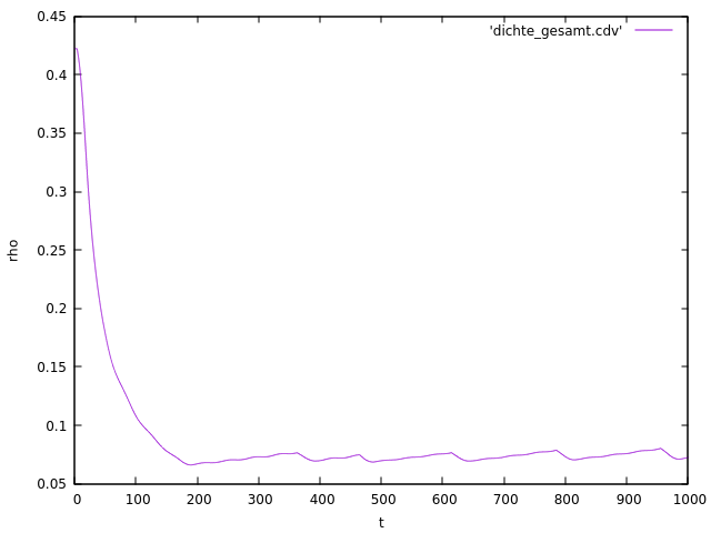
In our third setting all cars stand close to each other. We know this situation of traffic jam. The first car accelerates to a speed below the comfort flow value. This situation leads the drivers behind him to a well known scenario of everyday traffic. The traffic jam don't disperse homogeneously, there is rather a stop-and-go process where clusters of car groups (further small traffic jams) build. This can be seen this in the following plot (Figure 9), where the density of cars decreases in an exponential fashion.
We modified the following files.
Thanks to the tutors Laura Martin, Bulcsu Sandor and Hendrik Wernecke for support with technical and theoretical know-how!