by Yan Huck
Introduction
Snow Crystals exhibit a large range of geometries. Figure (1) shows a morphology diagram with the different snow crystals that develop
at different conditions. One characteristic property of the most snow flakes is their hexagonal symmetry. Of those, there are two configurations that can
be well described using a two dimensional model, the plates, which are almost full hexagons and the dendrites, which exhibit much more complex structures with
a wide range of different main arm and side arm branches.
However, the transition between those two is fluent.
Besides the attachement kinetics on the surface and thermodynamic processes in the environment, the
main factor that determines the growth of a snow crystal from a single ice seed is diffussive transport of the vapour inside the system. This phenomenon
is modelled by the diffusion equation (1).
\[\frac {\partial c}{\partial t} = D \nabla^2 c \qquad \quad \text{ (1)}\]
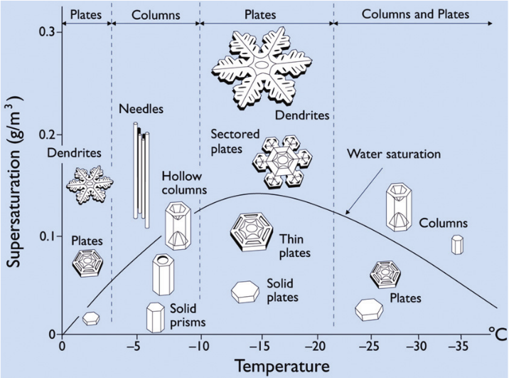
Figure 1: Morphology diagramm of snow crystals. It shows different crystal structures that emerge depending on the environmental conditions. Figure from [3].
Reiter's Model
A cellular automaton model that simulates the growth of two dimensional snow crystals such as plates and dendrites has been proposed by A. Reiter [1].
Since snow crystals generally exhibit hexagonal symmetry, this model uses a grid that is split into hexagonal cells. Every cell z has a continuous value st(z),
that resembles the amount of water stored in the cell. In the start of the simulation, this value is 1 for the cell in the middle, the seed,
and β for every other cell. The cells are grouped in different categories. The categorization is shown in figure (2). If st(z) >= 0, the cell is considered to be frozen.
A cell that is not frozen, but of which at least one of the nearest neighbours is frozen is a boundary cell. Frozen and boundary cells are receptive
cells. The others are non receptive cells. The cells at the border of the system are edge cells. In every step of the simulation two new variable
are defined for every cell: ut(z), which represents the amount of water in the cell that does participate in diffusion and vt(z), the amount
of water that is stored in the cell and doesn't participate in diffusion. The value of every cell z is progressively update by the
rules described below.
Hereby β defines the amount of water that is transported into the system by the edge cells. α is the diffusion
constant and characterices the distribution of the water inside the system. The constant γ describes water addition from a constant background
vapour. The idea of the model is that once a cell is receptive, it is attached to the crystal and can store the water that it contains. All other cells
don't store the water and underlie the diffusion. The diffusion is modelled by discretizing equation (1) on the hexagonal lattice.
Thereby the crystal can grow continously on the surface while the water gets transported there from the edge cells.
The canvas below shows an implementation
of this algorithm. The size of the system, namely the number of cells, and the parameters α, β and γ can be inserted via the input boxes. As a special feature,
another set of values can be inserted right next to the input boxes. By clicking 'c', the parameters change during the simulation. This can be regarded as a
simulation of a falling snowflake which crosses different environments while falling. Two further input boxes distinguish between a single initial seed
in the middle and a small cluster of seeds that resembles an imperfection which can occur in nature.
current state variables
If z is a receptive cell: \[u_{t}(z)=0 \quad \text{and} \quad v_{t}(z)=s_{t}(z)\]
If z is a non receptive cell: \[u_{t}(z)=s_{t}(z) \quad \text{and} \quad v_{t}(z)=0\]
variable update
For the receptive cells: \[v_{t+1}(z)=v_{t}(z)+\gamma\]
For every cell: \[u_{t+1}(z)=u_{t}(z)+\frac{\alpha}{2}(\overline{u_{t}(z)}-u_{t}(z))\]
For the edge cells: \[u_{t+1}(z)=\beta \quad \text{and} \quad v_{t+1}(z)=0\]
update st(z): \[s_{t+1}(z)=u_{t+1}(z) + v_{t+1}(z)=0\]
![Figure 2: Classification of the cells in the system. Figure from [2].](ClassificationCells.png)
Figure 2: Classification of the cells depending on position and value of st(z).
Analysis
The crystal growth and the resulting shape is sensitive to the choice of the parameters α, β and γ. Figure (3)
shows a few different crystals that develop for constant α and varying β and γ. The number of cells was 101 in those simulations. It is important to note that if γ=0, the resulting
shape will always be a full hexagon. The reason is that, once a cell is receptive, it is already frozen in the next step. There's no time to develop
a more complex structure with six main branches and side branches emerging from those, like in typical dendrite shapes.
The situation is different for a decreasing value of γ. The lower its value, the thinner are the main branches and the more complex
are the side branch structures. One might ask why this is the case, because a the first assumption could be that any cell thats gets receptive as soon
as it comes into contact with the surface, might as well be frozen a few times steps later. So why doesn't the growth always result in a full hexagon,
since every cell gets receptive once the surface has reached it. The reason lies in the underlying diffussive dynamics. Figure (4) shows different shapes emerging
for different values of the diffusion parameter. It can be seen that the lower the diffusion coefficient the more developed the side branch structures are.
An insight into this behaviour can be obtained by the Peclet number p (2). It compares the time scale of the diffusion transport to the time scale
of the crystal growth [3]. Empirical values for this quantity show that for many structures, especially
dendrites, diffusion adjusts the particle density around the crystal much faster than the shape changes[3]. This means that diffusion is the main determining factor for the growth. This phenomenon is
called "diffusion limited growth". It is a phenomenon encountered in different growth phenomena that
yields quite complex and self similar structues [4].
But why does it create such structures? A qualitative answer can be given by considering a flat growing
surface. If a bump appears on that smooth surface, it stands out further into the environment than the surrounding part. Consequently the particles
transported by diffusion reach the bump sooner than the flat surface which makes the bump bigger and thereby increases this effect. Therefore, once
a roughness develops on a flat surface it will continue to grow. This effect is known as the Mullins-Sekerka instability. To also get a quantitative understanding, consider a flat circle that grows
according to (1). The circle is perturbed by spherical harmonial function according to equation (3). A linear stability analysis then yields equation (4), in which
ks/kl is the ratio of thermal conductivities in the solid and the melted phase.
The instability occurs if the nucleation radius is bigger than than the critical radius R0. It depends on the
. The calculation is taken from [5].
Hence, the bigger the crystal gets, the more sensitive will it be to diffusion instabilities, resulting in a highly rough surface.
\[\tau_{diffusion}=\frac{R^{2}}{D}, \quad \tau_{growth}=\frac{2R}{v_{n}}, \quad p=\frac{R v_{n}}{2D} \qquad (2)\]
\[r=R+\delta Y_{lm}(\theta, \phi) \qquad (3) \]
\[R > R_{0}(l, \beta) = 1+(l+2)(l+\beta l +1)/2 \qquad (4) \]
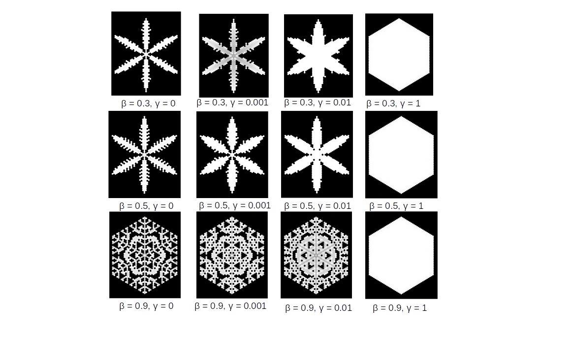
Figure 3: Crystal shapes emerging for different value of β and γ for α=1 and a system of 51 cells.
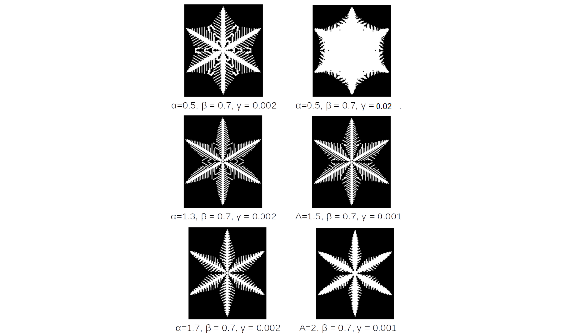
Figure 4: Crystal shapes emerging for different values of α in a system with 101 cells.
References
[1] A local cellular model for snow crystal growth
[2] Interface control and snow crystal growth
[3] The phyiscs of snow crystals
[4] Diffusion-limited aggregation: a kinetic critical phenomenon?
[5] Role of instabilities in determination of the shapes of growing crystals