Fitzhugh-Nagumo Reaction-Diffusion System

FitzHugh-Nagumo Model as a Reaction-Diffusion System

The FitzHugh-Nagumo model, named after Richard FitzHugh and J. Nagumo, who discovered it shortly after another, is a model that describes the reaction of a biological neuron when excited by an external stimulus $I_{ext}$. The differential equations describing the dynamical system are the following:
$$\begin{pmatrix}\dot{v}\\\dot{w} \end{pmatrix}=\begin{pmatrix}f(v,w)\\g(v,w)\end{pmatrix}= \begin{pmatrix} v-\frac{v^3}{3}-w+I_{e}\\\tau^{-1} (v-a-bw) \end{pmatrix}\tag{FN}$$
Where $v$ denotes the voltage on the membrane of the neuron and $w$ is a recovery variable.
It is a special case of the Van-der-Pol Oscillator $$\ddot{x}-\mu (1-x^2)\dot{x}+x = 0$$ which transforms into $$\begin{pmatrix}\dot{x}\\ \dot{y}\end{pmatrix}=\begin{pmatrix}\mu (x-\frac{x^3}{3} -y)\\ \frac{x}{\mu}\end{pmatrix}$$ for the Liénard-transformation $y = x-\frac{x^3}{3}-\frac{\dot{x}}{\mu}$. As one can see, the Van-der-Pol oscillator differs from the FitzHugh-Nagumo Model by the addition of two terms with constants $a\neq 0,\; b\neq0$ and a rescaling of $\dot{x}$.

For a system of neurons one can rewrite these equations as a reaction-diffusion system, by treating the discretized system of neurons as a continouus system, where a point in a $x\times y$ space corresponds to a neuron and holds a value $(v(x,y,t),w(x,y,t))$. The solution to the differential equations (and therefore the reaction to the excitation of a neuron) is a travelling voltage spike on the membrane of the neuron. For a system of neurons that are connected by axons, the spike of the voltage corresponds to a current that flows from neuron to neuron, generating patterns of excited neurons and not excited neurons. In the following simulation the neurons are pixels on a $300px \times 300px$ canvas who excite nearby neurons.

Diffusion

Diffusive systems are characterized by the Diffusion Equation $$\partial _t \rho(x,t) = D_\rho \Delta \rho(x,t).$$ This differential equation is solved by a wave equation of form $$\Phi (x,t) = \frac{1}{\sqrt{4 \pi Dt}}exp(\frac{-x^2}{4Dt}).$$ It has a Gaussian Form and runs in both directions. The same can be applied to the problem in $\mathbb{R}^2$.The FitzHugh-Nagumo model exhibits diffusion in form of such travelling wavfronts. The amplitude of the wave will be colour coded, where the colour red symbolizes a high excitation of a neuron and blue symbolizes a low excitation. When clicking on the canvas of the simulation, one excites the neurons around the mouse cursor. These neurons generate a spiking current that excites its surrounding neurons. The Fitzhugh-Nagumo Model can be seen as a reaction-diffusion system of following form: $$\tag{RD} \begin{pmatrix}\partial_ t \;v\\\partial_ t\; w\end{pmatrix} = \begin{pmatrix}D_v&0\\0& D_w\end{pmatrix}\begin{pmatrix}\Delta v \\ \Delta w\end{pmatrix}+ \begin{pmatrix} f(v,w)\\ g(v,w) \end{pmatrix}$$ Where the functions $f $ and $g $ are the right hand side functions of (FN).

Fixpoints, Turing Instabilities and Patterns

A fixpoint $x^*$ of a continouus dynamical system is a point in the phase space for which equation $$f(x^*)=0$$ holds. Furthermore a fix-manifold is manifold for which the fixpoint condition holds. The dimension of these manifolds can vary so they can be lines, areas, volumes and even higher dimensional shapes in the phase space. In the simulation the fix-manifolds are then the points of the phase space that stay excited or stay non-excited under time-transition. The simulation of the problem will be in $\mathbb{R}^2$ and the fix-manifolds will be of dimension $1$, ie. either closed or open lines. Fixpoints can either be stable, or unstable. A stable fixpoint is a fixpoint that attracts nearby points in the phase space while an instable fixpoint repels nearby points in the phase space. The stablility condition is given by $$|J(x^*)|\;\begin{cases}>0\; \mbox{for unstable manifolds}\\ <0 \;\mbox{for stable manifolds} \end{cases}\; ,$$ where $J$ denotes the Jacobi-Matrix of the dynamical system.
The key phenomenon that plays a role in pattern formation are Turing Instabilities. When two processes, who stabilize the system themselves are put into a system where they interact, the process of the entire system can turn out to be unstable and exhibit patterns. A Reaction-Diffusion System as (RD) follows a such dynamic. While Reaction and Diffusion lead to a spatially homogenous state, the interaction exhibit Turing patterns for certain parameters.
(RD) can be rewritten into $$\begin{pmatrix} \dot{v}\\ \dot{w}\end{pmatrix} = A_1\begin{pmatrix}v\\w\end{pmatrix} + A_2\begin{pmatrix}v\\w\end{pmatrix} = A\begin{pmatrix}v\\w \end{pmatrix}.$$Where $A_1 = diag(D_v\Delta,D_w\Delta)$ and $A_2=\begin{pmatrix}f_v&f_w\\g_v&g_w\end{pmatrix}$. And for a Fourier expansion of $v$ and $w$ is $A_1 = diag(-D_v k^2,-D_w k^2)$. A Turing Instability therefore occurs for $$|A_1|<0, \; |A_2|<0,\; |A|>0.$$ Or explicitly$$|A|=|f_w g_v|-(|f_v|+D_v k^2)(|g_w|-D_w k^2)>0.$$

Bifurcations

The dynamics of a dynamical system, their fixpoints and the stability fo the fixpoints can be dependent on the parameters of the system. A bifurcation happens when the system changes its dynamics when its parameters are changed. The patterns that a system forms will therefore change when input parameters are varied.

Simulation

Click on the canvas to excite neurons around the position of the cursor. Use the sliders to tweak the variables and observe the different patters that the system forms. Vary the parameter $a$ after a pattern has formed, not before. Pattern presets are starting points, there are many more patterns to be found when varying parameters after setting the starting points and the boundary conditions. Use the RGB sliders to change the colour scheme of the simulation.

These slider will change the parameters of the simulation:

a = 0

b = 0.9

I = 0

D_v = 0.45

D_w = 1.0

These sliders change the colour scheme of the simulation (RGB):

R = 0

G = 155

B = 210

You can select a preset parameter choices in the drop-down menu. The "wrap"-button activates /deactivates the boundary conditions, the "randomize"-button randomizes the values of each point in the mesh-grid. Different patterns emerge for different boundary conditions/initial conditions.

Code

The Laplacian was calculated by a function $laplace(u,x,y)$, where $x$ and $y$ are the coordinates for the current point in the ($resx\; \times\; resy$) mesh-grid. function laplace(u,x,y){ temp = 0; temp += u[mod(x+1,resx)][y]; temp += u[mod(x-1,resx)][y]; temp += u[x][mod(y+1,resy)]; temp += u[x][mod(y-1,resy)]; temp -= 4.*u[x][y]; return temp/dxsq; } Where a modulus function has been used to calculate the Laplacian on the edges of the grid. An important nuance: Unlike Python, arrays in Javascript can not handle negative entries of arrays ($dog[-1]$ is the last entry of the array $dog$ in Python). You can go around this issue by defining the modulus function as following: function mod(n,k){ return (n%k+k)%k; } The shift turns the negative value of the modulus operation into a positive one and by applying the modulus again, one makes sure that the result is in $\mathbb{Z}/k\mathbb{Z}$ for the case that $n\% k$ is not negative.
The algorithm used for solving the problem was Euler Inegration: $$\partial_t f = \frac{f(t+\Delta t)-f(t)}{\Delta t}$$ $$ f_{xy}^{t+1} = f_{xy}^{t}+\Delta t D \cdot \Delta f$$ Where $\Delta f$ is the laplacian from code above, or explicitly: $$\Delta f = \frac{f_{i+1,j}^t +f_{i-1,j}^t +f_{i,j+1}^t +f_{i,j-1}^t - 4f_{ij}^t}{\Delta x^2} $$ And D is the Diffusion-constant:$$D = \frac{\Delta x^2}{2\Delta t}$$

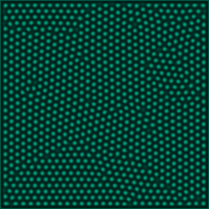
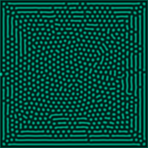
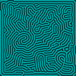
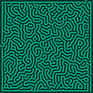
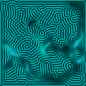
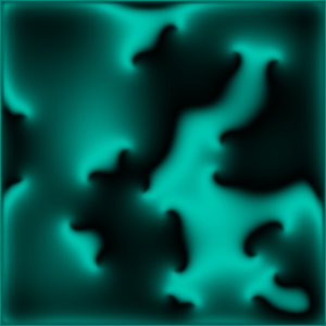
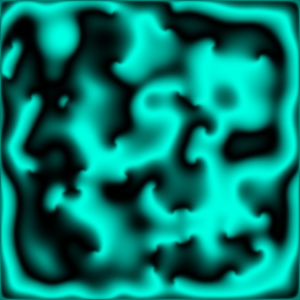
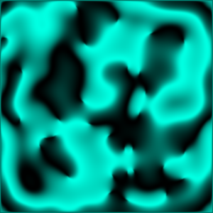
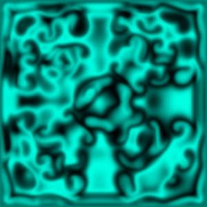
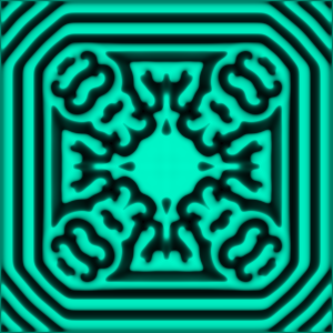
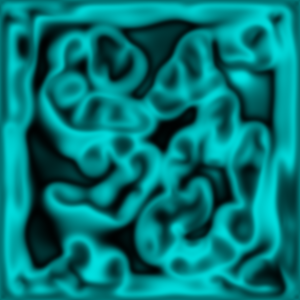
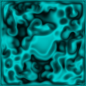
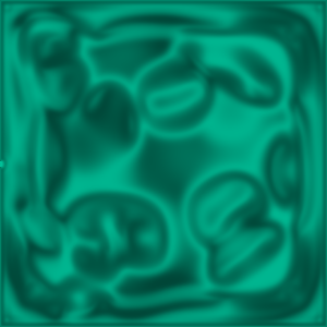
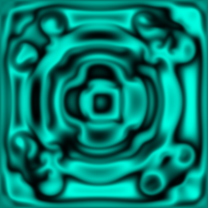
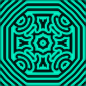
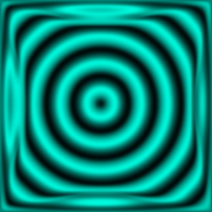
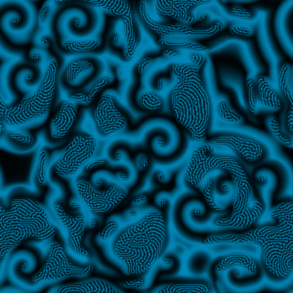
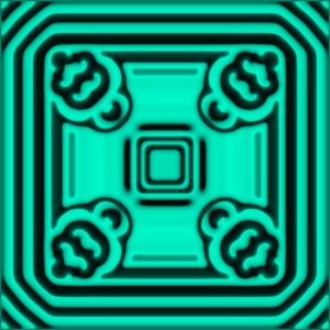
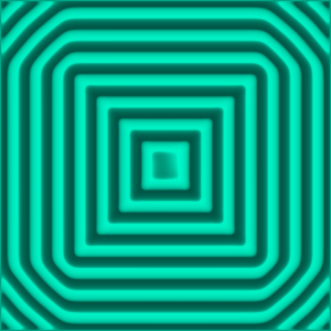
Patterns

References & further reading

[1] Encyclopedia of Computational Neuroscience: FitzHugh–Nagumo Model by William Erik Sherwood, University of Utah, Salt Lake City, UT, USA
[2] FitzHugh-Nagumo model, Eugene M. Izhikevich, http://www.scholarpedia.org/article/FitzHugh-Nagumo_model#fig:Nagumo_Circuit.gif

summer term 2020
Vasilios Mitsiioannou, mitsiioannou@itp.uni-frankfurt.de