Theory
The Gray-Scott system is defined by two equations that describe the behaviour of two reacting substances: \begin{align} \dot{u}&=-uv^2+F(1-u)+D_u\Delta u\\ \dot{v}&=uv^2-(F+k)v+D_v\Delta v \ .\\ \end{align} The variables in these equations \(u\) and \(v\) are the concentrations of the two reacting substances \(U\) and \(V\). On the left-hand side of each equation is the time derivative of one of these concentrations, describing the rate at which it changes. The right-hand sides of the equations both contain three separate terms . The first describes the reaction between the two substances. Since one \(U\) and two \(V\) react, the corresponding term includes \(u\) to the power of one and \(v\) to the power of two: \(uv^2\). As \(U\) gets consumed by the reaction, the term has a negative sign in the first equation. In the second equation it has a positive sign, as \(V\) is produced in the reaction.
The second term of the first equation describes the rate at which \(U\) is replenished externally. This is necessary, as \(U\) would otherwise simply be used up. The feed rate is given by the parameter \(F\). \(F\) is multiplied by \((1-u)\) to ensure that \(u\) is replenished at a rate dependent on the current concentration, which never exceeds \(1\). \(V\) does not need to be replenished, since it is produced in the reaction. Instead, it needs to be removed in order maintain the reaction. The rate of removal, the "kill rate", is controlled by the parameter \(k\). To remove \(V\) faster than \(U\) is added, \(k\) is added to \(F\) and multiplied by \(v\), since the removal of \(V\) is also supposed to be dependent on its concentration.
The last term in both equations describes the diffusion of \(U\) and \(V\), respectively.
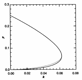
Phase diagram of the Gray-Scott system.[1]
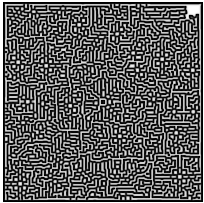
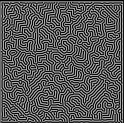
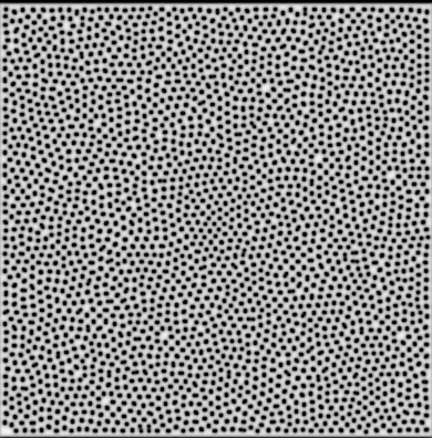
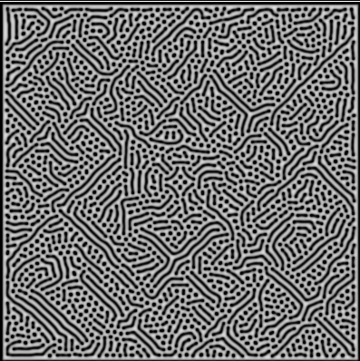
As you can see in the simulation above, there is a variety of patterns that can form for different values for \(F\) and \(k\). However, most possible combinations of values for those parameters lead to rather boring results: For combinations of \(F\) and \(k\) on one side of a certain threshold the screen is completely white, indicating that it is completely filled with substance \(U\). There is no substance \(V\) left to react with, and so the system is in equilibrium. The system will always return to this state.
For combinations of \(F\) and \(k\) on the other side of this threshold the screen completely fills with black. All of the added substance \(U\) reacts immediately, so the area is almost completely filled with substance \(V\). In this case the system is also in equilibrium, and will always return to this state.
The region of interest of the simulation is close to this threshold. The system changes from one stable state to the other. The system potentially has three fixed points: a trivial fixed point at \(u=1\) and \(v=0\), and two non-trivial fixed points . Which ones of these actually exists depends on the parameters \(F\) and \(k\). The trivial fixed point always exists, since the reaction cannot take place without \(v\). The two non-trivial fixed points exist beyond a bifurcation line at \(F=4(F+k)^2\) (the solid line in the figure). One of these is always a saddle, meaning it is stable in one direction and unstable in the other. The other one changes its stability at the dotted line. [2] These changes in number and stability of fixed points are what creates the patterns.
To the top