Introduction
In 1952, a year before American biologist James Watson and English physicist Francis Crick discovered DNA, Alan Turing, a British mathematician best known for his work on code-breaking and artificial intelligence, published his only one paper related to biology, “The chemical basis of morphogenesis”, which proposed a theory of how regularly repeating patterns are formed in nature. 1
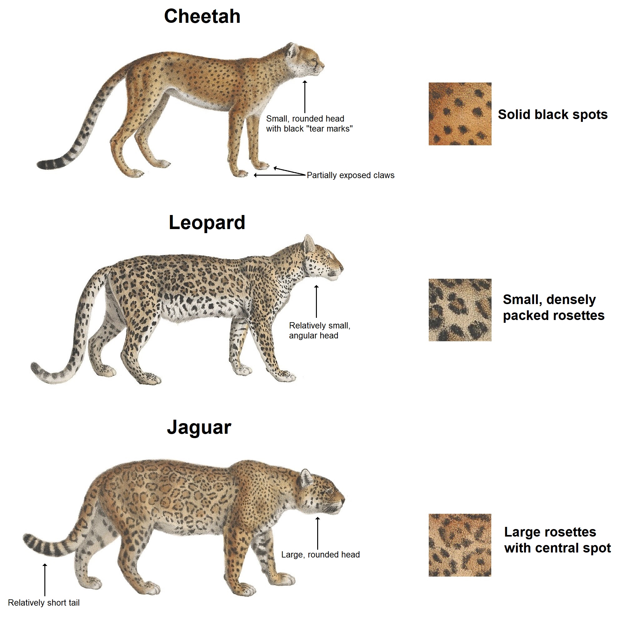
In this paper, he proposed a system consists of a number of chemicals diffusing through a mass of tissue of given geometrical form and reacting together within it. Although he did not apply his model to any specific biological situation, biologists are uncovering evidence of the patterning mechanisms that Turing proposed in his paper.3 People believe those countless varieties of stripes, spots and scales on vertebrates emerge from the interaction of two of these hypothetical chemical substances called “morphogens”.4
It is suggested that a system of chemical substances, called morphogens, reacting together and diffusing through a tissue, is adequate to account for the main phenomena of morphogenesis. — Alan Turing
The underlying mechanism that produces these observable spatial pattern is called Turing-type mechanism. Imagine two chemicals, u, called the activator, and v, called the inhibitor, diffuse in a closed system at different rates. Assume the diffusion coefficient of u, Du, and the diffusion coefficients of v, Dv are different.
where f(u,v) and g(u,v) denote the interation between these two morphogens. While these are called reaction-diffusion equations, we use Gray-Scott(GS) model, which was based on the Turing mechanism, to do the simulations. Notice that we are still working on a system with two kinds of chemicals. And we assume the chemical reactions to be:
P is an inert product of these irreversible reactions. By inputting a parameter k representing the rate of conversion of V to P, and a f representing the rate of the feeding process, the above equations could be transformed to reaction-diffusion equations in Gray-Scott model:
Methods
In this way, we are going to design a simulating system where we can choose different feed rates and death rates. We created a canvas of 700*400 pixels. By initialing a pixel with a value, 1 in this case, we can trigger the reaction. The diffusion is obtained by a laplace function. Renew values according to the previous values, this dynamical process is shown by using forward Euler integrations of the finite-difference equations5
  for (var x = 1; x < width - 1; x++) {
    for (var y = 1; y < height - 1; y++) {
      var a = grid[x][y].a;
      var b = grid[x][y].b;
      next[x][y].a = a + (dA * laplaceA(x, y)) - (a * b * b) + (feed * (1 - a));
      next[x][y].b = b + (dB * laplaceB(x, y)) + (a * b * b) - ((k + feed) * b);

      next[x][y].a = constrain(next[x][y].a, 0, 1);
      next[x][y].b = constrain(next[x][y].b, 0, 1);
    }
  }
- Here we use the simplest numerical integrator: Forward Euler method:
- $$ \frac {\partial x}{\partial t} = f(x, t), x(t=0) = x_0 $$ $$x_{t+1}=x_t+f_t {\Delta} t$$
- To obtain the function of the Laplace operator. We regard the values of a pixel with its neighboring pixels as elements in a 3X3 matrix A. Considering these values as the concentrations of the morphogens. For a grid cell(i, j), or a pixel, one possible implementation is to recognize its direct neighbors, i.e. (i, j-1),( i, j+1), (i-1, j), (i+1, j).
- $$ (\nabla^2 A)_{ij} = A_{i+1, j}+A_{i-1, j}+A_{i, j+1}+A_{i, j-1}-4A_{i, j}$$
However, it requires more iterations in processing. Instead, the Laplacian is performed by giving away the center weight(-1) to adjacent neighbors(+0.2) and diagonals(+0.05). $$ -A_{ij} \rightarrow A_{i+1, j}+A_{i-1, j}+A_{i, j+1}+A_{i, j-1}+4A_{i{\pm 1},j{\pm 1}}$$
Results
| Name | Feed Rate f | Death Rate k |
|---|---|---|
| Waves | 0.014 |
0.045 |
| Chaos | 0.026 |
0.051 |
| Spots and Loops | 0.018 |
0.051 |
| Moving Spots | 0.014 |
0.054 |
| Chaos and Holes | 0.034 |
0.056 |
| Mazes | 0.029 |
0.057 |
| Holes | 0.039 |
0.058 |
| Pulsating Solitons | 0.025 |
0.060 |
| The U-Skate World | 0.062 |
0.06093 |
| Worms | 0.078 |
0.061 |
| Solitons | 0.030 |
0.062 |
Reference
1. Jennifer Ouellette, "Biologists Home In on Turing Patterns", March 25, 2013, https://www.quantamagazine.org/biologists-home-in-on-turing-patterns-20130325/. ↩
2. Jean Charles Werner, “Cheetah, leopard & jaguar (en).jpg”, From Wikimedia Commons, the free media repository, November 14, 2018 https://commons.wikimedia.org/wiki/File:Cheetah,_leopard_%26_jaguar_(en).jpg. ↩
.jpg)
3. Jonathan Lambert, “Ancient Turing Pattern Builds Feathers, Hair — and Now, Shark Skin”, January 2, 2019, https://www.quantamagazine.org/ancient-turing-pattern-builds-feathers-hair-and-now-shark-skin-20190102/. ↩
4. J. D. Murray, “Why Are There No 3-Headed Monsters? Mathematical Modeling in Biology”, https://pdfs.semanticscholar.org/4572/1b7d2bfd04e273c84d9d2c762ac506edd97f.pdf. ↩
5. John E. Pearson, “Complex Patterns in a Simple System”, http://rocs.hu-berlin.de/complex_sys_2017/resources/Papers/pearson_1993.pdf. ↩
Simulator
Instructions
- Click Play/Pause button to start or pause the simulation
- Either paint directly on the canvas or click Random button to initialize
- One can also reset the canvas by clicking Clear button
- Use the sliders to set the values of the Feed rate k and the Death rate k, or type in the last two digits in the textboxes
- Google Chrome is always better