Display of Pattern Formation using the Gierer-Meinhardt Model
Elias Fischer and Stefanie Mrozinski
Abstract
Reaction-diffusion systems as introduced by Alan Turing consider possible interaction of two chemical reactants with different diffusion rates. cf. [2] However, this model explains the generation of local maxima, but it is not able to explain pattern-forming capability. cf. [2] Introducing a interaction between a short range activator and a long range inhibitor the Gierer-Meinhardt-Model shows pattern formation from a more or less homogenous initial situation. As the activator up-regulates the inhibitor and the inhibitor down-regulates the activator Turing instabilities can occur and lead to spatial patterning. cf. [1] The occurence of stripe-like patterns can however be only achieved by implementing an additional saturation term in the model. cf. [2]
Our aim is to implement the Gierer Meinhardt Model with an additional saturation term in a graphical window and ensure the regulation of parameters.
Table of contents
Model and Theory
The interaction of molecules plays a crucial role in the theory of biological pattern formation. As a mathematical description one needs to describe changes of concentration in time and space as a function of the local concentration of the substances. For an array of cells, which describes the local changes of the activator and inhibitor per time, the Gierer Meinhardt model can be written as follows:[2] $$ {\partial a\over \partial t} = {\rho \left({a^2\over h} - \mu a \right) + D_a \Delta a}$$ $$ {\partial h\over \partial t} = {\rho \left( a^2 - \nu h \right) + D_h \Delta h}$$ \( \Delta \) represents the Laplace-Operator. The first equation shows the time evolution of the activator which is proportional to the production term \(a^2\). As the production of the activator is dependent on the concentration of the inhibitor one regulates the kinetics with the additional term \( 1\over h \). Additionally the inhibitor has to spread more rapidly than the activator. This can be achieved with the condition \( D_a \ll D_h \) cf.[2] The homogenous distribution becomes unstable for a small increase of the activator concentration as it is increasing further due to the autocatalysis of the activator. On the contrary, the inhibitor is diluting faster into the cell which leads to a decrease of the autocatalysis in this regions. Therefore, one obtains a new patterned steady state when a high activator concentration is in a dynamical equilibrium with the surrounding inhibitor distribution.
Stripe-like patterns as one can see in organisms such as zebrafish or in spacing of leaves emerge for an upper bound of the activator production. Therefore one can extend the prior introduced equations as follows: [2] $$ {\partial a\over \partial t} = {\rho \left( {a^2 \over h(1+\kappa a^2)} - \mu a \right) + D_a \Delta a}$$ $$ {\partial h\over \partial t} = {\rho \left( a^2 - \nu h \right) + D_h \Delta h}$$ The added \( \kappa \) ensures the stripe like pattern as it leads to self-enhancing reaction and an upper limit of activator production. By implementing \( \kappa\) one pays attention to cell-regulating properties as the size regulation and the spacing of structure which makes this model more suitable for biological systems. cf. [2]
The identification of the occurence of Turing instability is crucial for the prediction of pattern formation. To examine the stability of the above shown systems one has to linearize the equations. As [1] has shown one obtains a coexistant equilibrium for \( E^* = (a^*, h^*) \) = \( (a^*, {(a^*)^2\over \mu}) \). Moreover, one can predict that the equilibrium only exists above \( a^* = {\mu \over \nu} \).
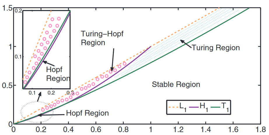
The figure shows Hopf and Turing bifurcations in the plane of \( a^* , {\mu \over \nu} \). cf. [1] In between L1 which represents the dividing line of the coexisting equilibrium and H1 and T1 patterns can be formed. cf. [1]
The approximation of pattern formation by diffusion already demonstrates pattern formation ability. However the simulation of real biological systems has to consider gene expression, a chain of different molecules, ligand secretion, different receptors and transfer components of the cell. cf.[3]
Simulation
The upper graphical window shows the activator distribution and concentration. As the activator is dependent on the time evolution of the inhibitor the concentration and distribution of it are also presented in the lower window. Before starting the simulation one needs to distribute the activator concentration via clicking on the graphical surface or choosing the randomize button. Once the activator is spread one can start to see the evolution of the process by clicking start. While the simulation is running, a parameter change is possible and becomes effective.
The color code helps to differentiate between different concentrations of the inhibitor and the activator. Red represents the highest concentration. Fading into yellow, green, blue and black the concentration of the different reactants decreases. The values in the box represent the value of the substance at which it is assigned the respective colour. To function properly, the values have to increase from left to right. If you want to see a color gradient with only a single color, tick the tickbox. The values max(a) and max(h) represent the current highest value of the activator and inhibitor.
Parameters
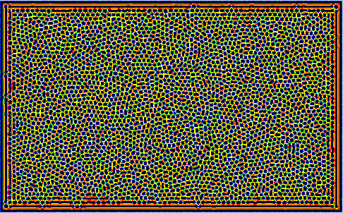
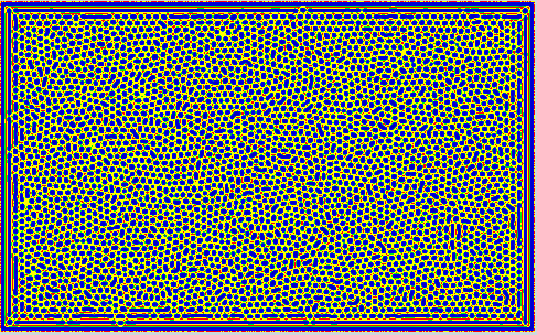
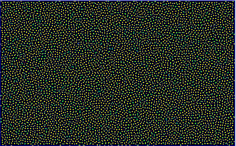
Results
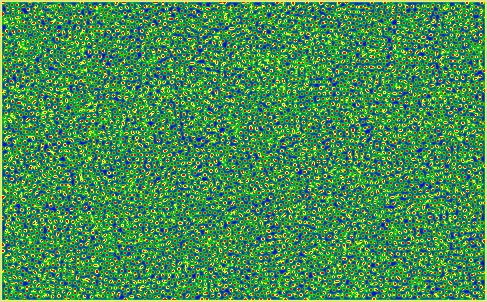
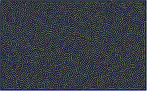
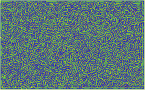
Some Snapshots of the time evolution of the activator and inhibitor with the 3 different presets of parameters are presented here at a higher resolution. These configurations are achieved by selecting a preset and pressing randomize before starting the simulation. This puts the system to the respective fix point, but an additional pertubation is introduced by adding a small random value to each cell. Then you have to wait a while until the reaction has slowed down sufficiently.
References
[1] Yongli Song et al., Pattern dynamics in Gierer-Meinhardt model with saturating term, Elsevier 2017.