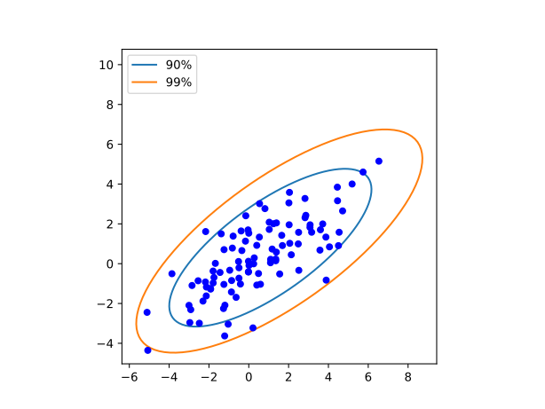
#!/usr/bin/env python3
import math                      # math
import numpy as np               # numerics
import matplotlib.pyplot as plt  # plotting
from numpy import linalg as LA   # linear algebra

# flip to True to print intermediate values
DEBUG = False

# ***
# *** covariance matrix from data
# ***

def covarianceMatrix(data):
  '''Normalized (divide-by-N, population)
     covariance matrix of input data.
     Alternatives to manual loop:
     np.mean(data, axis=0) and
     np.cov(data.T, bias=True).'''
  nRow = len(data)                     # number of data points
  nCol = len(data[0])                  # dimension
  mean = np.zeros(nCol)                # empty array
  for thisRow in data:                 # loop over data points
    mean += thisRow*1.0/nRow           # vector-mean
#
  coVar = np.zeros((nCol,nCol))        # empty matrix
  for thisRow in data:
    dataPoint = thisRow - mean         # shifted data point
    coVar += np.outer(dataPoint,dataPoint)/nRow  # outer product
#
  if DEBUG:
    print("\ninput data\n", data)
    print("nRow, nCol\n", nRow, nCol)
    print("mean\n", mean)
  print("\n covariance matrix: measured \n",coVar)
#
  return mean, coVar                   # returning both

# ***
# *** generate data for plotting an ellipse
# ***

def plotEllipseData(data):
  """generates ellipse from symmetric 2x2 slice
   of the input matrix"""
#
# slice (copy: don't mutate caller's matrix)
  slice22 = data[:2, :2].copy()
# eigh: for symmetric matrices
  eigenValues, eigenVectors = LA.eigh(slice22)
#
  if (eigenValues[0]<0.0) or (eigenValues[1]<0.0):
    print("# plotEllipseData: only positive eigenvalues (variance)")
    return
#
  if DEBUG:
    print("\n# slice22     ", slice22)
    print("\n# eigenValues ", eigenValues)
    print("\n# eigenVectors\n",eigenVectors)
#
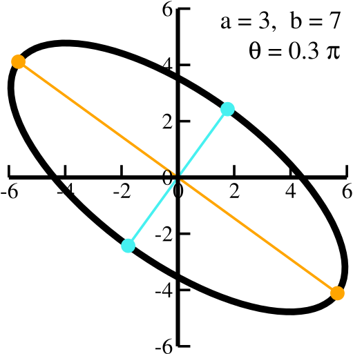
  a = math.sqrt(eigenValues[0])
  b = math.sqrt(eigenValues[1])
# first eigenvector = eigenVectors[:, 0]
  cTheta = eigenVectors[0, 0]
  sTheta = eigenVectors[1, 0]
  x = []
  y = []
  for i in range(nPoints:=101):          # walrus assignment
    tt = i*2.0*math.pi/(nPoints-1)       # full loop
    cc = math.cos(tt)
    ss = math.sin(tt)
    xx = a*cTheta*cc - b*sTheta*ss
    yy = a*sTheta*cc + b*cTheta*ss
    x.append(xx)
    y.append(yy)
#   print(xx,yy)
  return x, y

# ***
# *** generate 2D test data
# ***

def testData(angle, var1, var2, nData, startMean=(0.0,0.0)):
  r"2D Gaussian for a given angle and main variances.\
   A = \sum_i \lambda_i |lambda_i><lambda_i|"
#
  eigen1 = [math.cos(angle),-math.sin(angle)]
  eigen2 = [math.sin(angle), math.cos(angle)]
  startCoVar  = var1*np.outer(eigen1,eigen1)
  startCoVar += var2*np.outer(eigen2,eigen2)
  print("\n covariance matrix: data generation \n",startCoVar)
  return np.random.multivariate_normal(startMean, startCoVar, nData)

# ***
# *** main (with a block)
# ***

if (__name__ == "__main__"):    # blocking out-of-use access
#
  np.random.seed(0)             # reproducible test data

  dataMatrix = testData(0.3*math.pi, 1.0, 9.0, 100)
  mean, coVar = covarianceMatrix(dataMatrix)

  if DEBUG:
    print("\n#main: data\n", dataMatrix)
    print("#main: mean\n", mean)
    print("\n#main: coVar matrix \n",coVar)

  xEllipse, yEllipse = plotEllipseData(coVar)  # coVar-ellipse

  xData = [thisRow[0] for thisRow in dataMatrix]
  yData = [thisRow[1] for thisRow in dataMatrix]

  Z_90 = math.sqrt(4.605)       # 90% confidence (chi2, 2 dof)
  Z_95 = math.sqrt(5.991)       # 95% confidence
  Z_99 = math.sqrt(9.210)       # 99% confidence
#
  xE_90 = [Z_90*xx + mean[0] for xx in xEllipse]
  yE_90 = [Z_90*yy + mean[1] for yy in yEllipse]
  xE_95 = [Z_95*xx + mean[0] for xx in xEllipse]
  yE_95 = [Z_95*yy + mean[1] for yy in yEllipse]
  xE_99 = [Z_99*xx + mean[0] for xx in xEllipse]
  yE_99 = [Z_99*yy + mean[1] for yy in yEllipse]
#
  plt.plot(xE_90, yE_90, label="90%")
  plt.plot(xE_95, yE_95, label="95%")
  plt.plot(xE_99, yE_99, label="99%")
  plt.plot(xData, yData, "ob", markersize=5)
#
  plt.legend(loc="upper left")
  plt.axis('square')                           # square plot
  plt.title("Confidence ellipses from sample covariance")
  plt.xlabel("x")
  plt.ylabel("y")
  plt.savefig('foo.svg')                       # export figure
  plt.show()