Getting started 

(1.1)

(1.2)

(1.3)

Symbolic Calculations 

Definition of Variables and Functions 

>

A:=3;

 

(2.1.1)

 

>

A+2;

 

(2.1.2)

 

>	f:=(x)->sqrt(x);

 

(2.1.3)

 

>

f(4);

 

(2.1.4)

 

>	g:=(x,y)->sin(x)+cos(y);

 

(2.1.5)

 

>	g(Pi/2,0);

 

(2.1.6)

 

Simplification of expressions 

>	Exp1:=f(x)*(x^(5/2)+x^(3/2));

 

(2.2.1)

 

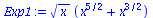>	expand(Exp1);

 

(2.2.2)

 

>	Exp2:=sin(x)^2+cos(x)^2;

 

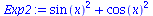(2.2.3)

 

>	simplify(Exp2);

 

(2.2.4)

 

Symbolic differentiation and integration 

>	diff(f(x),x);

 

(2.3.1)

 

>	int(f(x),x);

 

(2.3.2)

 

>	int(f(x),x=0..5);

 

(2.3.3)

 

>	diff(g(x,y),x);

 

(2.3.4)

 

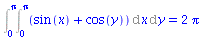
>	int(int(g(x,y),x=0..Pi),y=0..Pi);

 

(2.3.5)

 

>	Int(Int(g(x,y),x=0..Pi),y=0..Pi)= int(int(g(x,y),x=0..Pi),y=0..Pi);

 

(2.3.6)

 

Solving algebraic equations 

>	Eq1:=x^2-3*x+1=0;

 

(2.4.1)

 

>	solve(Eq1,x);

 

(2.4.2)

 

>	evalf(solve(Eq1,x));

 

(2.4.3)

 

Solving ordinary differential equations 

>	DGL1:=diff(x(t),t)=3*x(t);

 

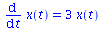(2.5.1)

 

>	dsolve(DGL1,x(t));

 

(2.5.2)

 

>	dsolve({DGL1,x(0)=10},x(t));

 

(2.5.3)

 

Numerical Calculations 

Limit finding 

>	Limit(sin(x)/x,x=0)=limit(sin(x)/x,x=0);

 

(3.1.1)

 

Minimum (maximum) of lists 

>	List:={2,32,13,7};

 

(3.2.1)

 

>	min(List);

 

(3.2.2)

 

>	max(List);

 

(3.2.3)

 

Interpolation 

>	with(Statistics):

 

>	Xvalues:=[0,1,2,3,4];

 

(3.3.1)

 

>	Yvalues:=[0.2,0.98,4.1,8.8,17];

 

(3.3.2)

 

>	Fit(a+b*x^2, Xvalues, Yvalues, x);

 

(3.3.3)

 

Numerical integration 

>	int(1/exp(x*ln(x)), x=1..infinity);

 

(3.4.1)

 

>	evalf(int(1/exp(x*ln(x)), x=1..infinity));

 

(3.4.2)

 

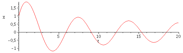
Solving ordinary differential equations 

>	DGL2:=(t+1)^2*(diff(x(t),t,t))+(t+1)*(diff(x(t),t))+((t+1)^2-0.25)*x(t) = 0;

 

(3.5.1)

 

>	Ergebnis:=dsolve({DGL2, x(0) = 1, (D(x))(0) = 2}, type=numeric,output=listprocedure);

 

(3.5.2)

 

>	with(plots):

 

>	odeplot(Ergebnis,[t,x(t)],0..20,numpoints=1000);

 

 

Visualisation of Data 

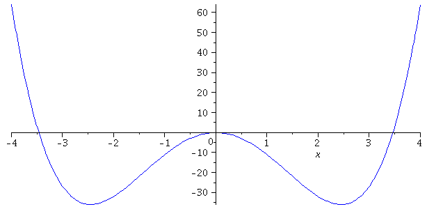
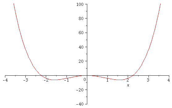
2D plots 

>	f:=(x)->x^4-12*x^2; plot(f(x),x=-4..4,color=blue);

 

 

 

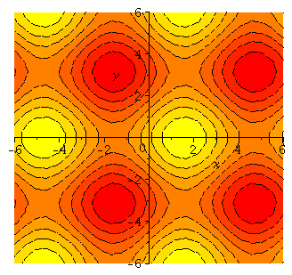
Contour plots 

>	with(plots): f:=(x,y)->sin(x)+cos(y); contourplot(f(x,y),x=-6..6,y=-6..6,filledregions = true);

 

 

 

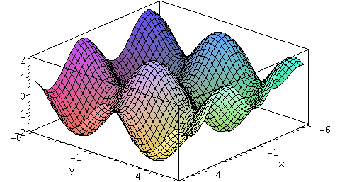
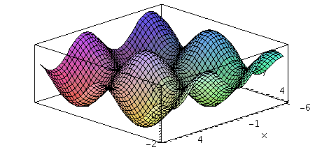
3D surface plots 

>	plot3d(f(x,y),x=-6..6,y=-6..6,axes=boxed,numpoints=1500);

 

 

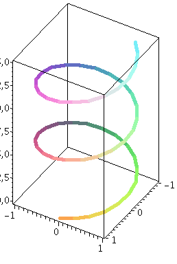
Spacecurves 

>	spacecurve([cos(t), sin(t), t], t = 0 .. 15,axes=boxed,thickness=3);

 

 

Animations 

>	f:=(x,a)->x^4-a*x^2; animate(f(x,a),x=-4..4,a=5..12,view=[-4..4,-40..100]);

 

 

 

>	f:=(x,y,t)->sin(x)+cos(t*y); animate3d(f(x,y,t),x=-6..6,y=-6..6,t=1..2,axes=boxed,numpoints=2000);

 

(4.5.1)

 

(4.5.1)

 

Programming tools 

Loops 

>	a:=1: for i from 1 by 1 to 10 do a:=a*i: od: a;

 

(5.1.1)

 

>	factorial(10);

 

(5.1.2)

 

If procedures 

>	a:=12: b:=34: if b < a then print("a is greater than b") else print("a is not greater than b") end if:

 

(5.2.1)

 

Examples