Visual transformer on MNIST

Creating the model

The following program is based on the code example "Image classification with Vision Transformer"[4] and has been modified to work with the MNIST dataset. An overview of the (relative) use of computing resources for training and the accuracy depending on the hypermarameters is provided in a later chapter.

Loading the datasets


import numpy as np
import tensorflow as tf
from tensorflow import keras
from tensorflow.keras import layers
import tensorflow_addons as tfa

# Define a function to change the MNIST label dimension
def change_to_right(wrong_labels):
    right_labels=[]
    for x in wrong_labels:
        for i in range(0,len(wrong_labels[0])):
            if x[i]==1:
                right_labels.append(i)
    return right_labels

# Model / data parameters
num_classes = 10
input_shape = (28, 28, 1)

# Load the data and split it between train and test sets
(x_train, y_train), (x_test, y_test) = keras.datasets.mnist.load_data()

# Scale images to the [0, 1] range
x_train = x_train.astype("float32") / 255
x_test = x_test.astype("float32") / 255

# Make sure images have shape (28, 28, 1)
x_train = np.expand_dims(x_train, -1)
x_test = np.expand_dims(x_test, -1)

# Convert class vectors to right format
y_train = tf.convert_to_tensor(np.array(change_to_right(keras.utils.to_categorical(y_train, num_classes))))
y_test = tf.convert_to_tensor(np.array(change_to_right(keras.utils.to_categorical(y_test, num_classes))))

Configuring the hyperparameters


learning_rate = 0.001
weight_decay = 0.0001
batch_size = 2000
num_epochs = 100

The learning rate is a hyperparameter that controls the step size at which the optimizer makes updates to the model's parameters during training. It determines how fast or slow the optimizer (here: Adam) learns from the data: A small learning rate means that the optimizer makes small updates to the model's parameters with each iteration, which can lead to slow, but stable convergence. A high learning rate results in larger updates and faster convergence, but can cause the optimizer to oscillate or miss the optimal solution.

Weight decay is a regularization technique used to prevent overfitting in neural networks by adding a penalty term to the loss function that encourages the model to have smaller weights. This results in simpler and more generalizable models. It will be used in combination with data augmentation (see next sub-chapter) to prevent overfitting, resulting in a more generalizable model.

The batch size is the number of samples used in each iteration of the training process. A larger batch size can make the training process faster and more stable, but will also require more RAM. After using the full RAM, the significantly slower Swap partition will be used, negating the faster processing speed. When a significant amount of memory is in swap, the computer might freeze temporarily. It is advisable to start with a low num_epochs (e.g. 1), the number of learning cycles with full dataset, to keep the downtime to a minimum.


image_size = 28  # We'll resize input images to this size
patch_size = 14  # Size of the patches to be extract from the input images
num_patches = (image_size // patch_size) ** 2
projection_dim = 96
num_heads = 4
transformer_units = [
    projection_dim * 2,
    projection_dim,
]  # Size of the transformer layers
transformer_layers = 16
mlp_head_units = [2048, 1024]  # Size of the dense layers of the final classifier

The image size is the (desired) width and height of the image in pixel. Setting this to another value than the original image size and using the corresponding function below will result in a resized image, which allows the usage of a larger set of patch sizes. The patch size is the size of the sub-matrices the image will be divided into, to be given to the transformer. A larger patch size allows the model to see more of the image at once, which can provide more contextual information, with an increase in computational resources needed. Smaller patches allow the model to recognize local features and be less dependent on the background. With the dataset used, larger patch sized should get better results, as the digits lack local features and backgrounds.

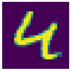
This 4 out of the MNIST training set has been resized to 32x32 pixel and divided into patches of 6x6.

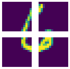
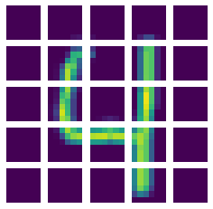
This 6 out of the MNIST training set with a size of 28x28 pixel has been divided into patches of 14x14.

The projection dimension controls the dimensionality of the internal representations used. In particular, it determines the size of the vectors that represent the image patches and the features extracted from them. Increasing the projection dimension and thus using lagrer vectors leads to increased processing time and RAM requirements, but allows the model to represent more complex features. The same applies for the number of transformer layers, as the ouput of each layer is fed into the next one to allow the model to understand more complex relations.

Data augmentation


data_augmentation = keras.Sequential(
    [
        layers.Normalization(),
        #layers.Resizing(image_size, image_size),
        #layers.RandomFlip("horizontal"),
        layers.RandomRotation(factor=0.02),
        layers.RandomZoom(
            height_factor=0.2, width_factor=0.2
        ),
    ],
    name="data_augmentation",
)
# Compute the mean and the variance of the training data for normalization.
data_augmentation.layers[0].adapt(x_train)

Data augmentation is a technique used in machine learning to increase the size of the training dataset by applying various transformations to the original data. The goal of data augmentation is to increase the variability of the training dataset to train more accurate and robust models with the same amount of labeled data. There are various data augmentation techniques:

Flipping: Horizontally or vertically flipping the image. This was not used, as it might decrease accuracy in distinguishing 6 from 9.
Rotation: Rotating the image by a certain degree. This might simulate writing at different angles or switching hands and is therfore used.
Scaling: Zooming by a certain factor. This was used.
Translation: Shifting the image by a certain amount. This was not used.
Color manipulation: Changing the brightness, contrast, or saturation of the image. For normalized scans, this should be irrelevant.
Noise injection: Adding random noise to the image. This was not used; however there exists a different dataset (Corrupted MNIST), which might benefit from it.


def mlp(x, hidden_units, dropout_rate):
    for units in hidden_units:
        x = layers.Dense(units, activation=tf.nn.gelu)(x)
        x = layers.Dropout(dropout_rate)(x)
    return x

class Patches(layers.Layer):
    def __init__(self, patch_size):
        super().__init__()
        self.patch_size = patch_size

    def call(self, images):
        batch_size = tf.shape(images)[0]
        patches = tf.image.extract_patches(
            images=images,
            sizes=[1, self.patch_size, self.patch_size, 1],
            strides=[1, self.patch_size, self.patch_size, 1],
            rates=[1, 1, 1, 1],
            padding="VALID",
        )
        patch_dims = patches.shape[-1]
        patches = tf.reshape(patches, [batch_size, -1, patch_dims])
        return patches

class PatchEncoder(layers.Layer):
    def __init__(self, num_patches, projection_dim):
        super().__init__()
        self.num_patches = num_patches
        self.projection = layers.Dense(units=projection_dim)
        self.position_embedding = layers.Embedding(
            input_dim=num_patches, output_dim=projection_dim
        )

    def call(self, patch):
        positions = tf.range(start=0, limit=self.num_patches, delta=1)
        encoded = self.projection(patch) + self.position_embedding(positions)
        return encoded

def create_vit_classifier():
    inputs = layers.Input(shape=input_shape)
    # Augment data.
    augmented = data_augmentation(inputs)
    # Create patches.
    patches = Patches(patch_size)(augmented)
    # Encode patches.
    encoded_patches = PatchEncoder(num_patches, projection_dim)(patches)

    # Create multiple layers of the Transformer block.
    for _ in range(transformer_layers):
        # Layer normalization 1.
        x1 = layers.LayerNormalization(epsilon=1e-6)(encoded_patches)
        # Create a multi-head attention layer.
        attention_output = layers.MultiHeadAttention(
            num_heads=num_heads, key_dim=projection_dim, dropout=0.1
        )(x1, x1)
        # Skip connection 1.
        x2 = layers.Add()([attention_output, encoded_patches])
        # Layer normalization 2.
        x3 = layers.LayerNormalization(epsilon=1e-6)(x2)
        # MLP.
        x3 = mlp(x3, hidden_units=transformer_units, dropout_rate=0.1)
        # Skip connection 2.
        encoded_patches = layers.Add()([x3, x2])

    # Create a [batch_size, projection_dim] tensor.
    representation = layers.LayerNormalization(epsilon=1e-6)(encoded_patches)
    representation = layers.Flatten()(representation)
    representation = layers.Dropout(0.5)(representation)
    # Add MLP.
    features = mlp(representation, hidden_units=mlp_head_units, dropout_rate=0.5)
    # Classify outputs.
    logits = layers.Dense(num_classes)(features)
    # Create the Keras model.
    model = keras.Model(inputs=inputs, outputs=logits)
    return model

Running the experiment

The next step is to train and test the model. All results have to be taken with a grain of salt: Background tasks have a huge impact if the computing power is low and generally, more epochs would have been needed to converge to the possible accuracy. Some of the earlier runs have had horitonal flips.


def run_experiment(model):
    optimizer = tfa.optimizers.AdamW(
        learning_rate=learning_rate, weight_decay=weight_decay
    )

    model.compile(
        optimizer=optimizer,
        loss=keras.losses.SparseCategoricalCrossentropy(from_logits=True),
        metrics=[
            keras.metrics.SparseCategoricalAccuracy(name="accuracy"),
            keras.metrics.SparseTopKCategoricalAccuracy(5, name="top-5-accuracy"),
        ],
    )

    checkpoint_filepath = "/tmp/checkpoint"
    checkpoint_callback = keras.callbacks.ModelCheckpoint(
        checkpoint_filepath,
        monitor="val_accuracy",
        save_best_only=True,
        save_weights_only=True,
    )

    history = model.fit(
        x=x_train,
        y=y_train,
        batch_size=batch_size,
        epochs=num_epochs,
        validation_split=0.1,
        callbacks=[checkpoint_callback],
    )

    model.load_weights(checkpoint_filepath)
    _, accuracy, top_5_accuracy = model.evaluate(x_test, y_test)
    print(f"Test accuracy: {round(accuracy * 100, 2)}%")
    print(f"Test top 5 accuracy: {round(top_5_accuracy * 100, 2)}%")

    return history


vit_classifier = create_vit_classifier()
history = run_experiment(vit_classifier)

At first, the image and patch sizes have been varied. batch_size = 128; layers = 8; epochs = 1; projection_dim = 48.

Image size	Patch size	Accuracy [%]	Training time [s]
48	6	94,91	412
56	7	93,96	414
32	6	95,59	165
64	12	94,93	166
32	8	94,62	97
28	7	93,72	96
21	7	93,43	72
28	4	94,68	313

Generally, more patches seem to be more computationally demanding. The best accuracy was achieved with a combination of parameters that leads to edges being cut off.

For fixed image (28x28) and patch(7x7) size, the projection dimension is varied:

Projection dimension	Accuracy [%]	Training time [s]
64	93,78	122
48	93,59	95
32	93,38	82
16	91,33	63

Higher projection dimension gives more accuracy, but requires more processing time.

Other values for the hyperparameteres have been tested; The best accuracy (98,94%) in the serie was achieved in under 2 hours with:
Epochs: 100
Batch size: 2000
Layers: 16
Image size: 28 (not resized)
Patch size: 14 (4 Patches)
Projection dimension: 96

This result has both worse accuracy and a longer compute time than the basic CNN example from keras.io (>99%, 2,5min).

Visual transformer and the MNIST dataset

Introduction

Transformers

MNIST database

Creating the model

Loading the datasets

Configuring the hyperparameters

Data augmentation

Running the experiment

Resources