What do we want to achieve
Let's suppose we got some input data $X$ that we want to classify by our own chosen classes. Our task is now to set up an model which our computer
can use to predict the classes. This is done by defining two important functions called the score function $F(X;W,b)$ and the Loss function $L(F)$. The score function includes
our model paramteres called Weights $W$ and biases b and takes the input data to compute a class score for the input. The loss function measures the agreement between the predicted
scores of the score function and the ground thruth level of the input data. The classification prozedure then reduces to an optimization problem where the loss function is to
minimize with respect to the parameters we put in our model.
Note: The input data $X$ remains unchanged during the optimization but our paramters, Weights $W$ and biases $b$, will change until the desired loss is achieved.
The basic calculations of a neuron
In our case of deep learning the score function will be represented as a convolutional neural network(ConvNet), where every neuron in the system behaves in the same functional way.
Every neuron has its associated weights which it uses to calculate a weighted sum of the input Data and adds its bias to this sum. Finally the neurons takes this expression and
uses some non-linear function on it which we call activation function. The output of the activation function is considered to be the signal firing of the neuron. The non-linearity
of the activation function is crucial for the model and brings in complexity.In our case we will use the rectified linear unit function (RELU-function),
which threshholds the output to positive values.
The RELU function: $f(x)=max(0,x)$.

Branislav Gerazov, CC BY-SA 4.0, via Wikimedia Commons
The method used in deep learning
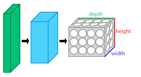
As mentioned our aim is to implement a convolutional neural network as score function which takes our input data, in our case pictues in pixel, as input and puts out a class score for every picture. For a convolutional neural network the layers are realized as volumes of neurons. we will stack the pixels of every color channel along the depth dimension of our input volume.
the convolutional neural network
Convolutional neural networks (ConvNet) almost share the same architecture as neural networks. The neurons in ConvNets are arranged in Layers which have three dimensions
$(Width \times Height \times Depth)$. The neurons of the first Layer of a ConvNet refer to the input Data and the neurons of the last layer to the output of the network.
Layers inbetween, called hidden Layers, are implemented to process the Data in a non-linear manner. There are several types of hidden Layers which will be shortly introduced.
Aphex34, CC BY-SA 4.0, via Wikimedia Commons
Note: The loss-function will only be put on the last layer of the ConvNet since the last layer holds the predictions of the network.
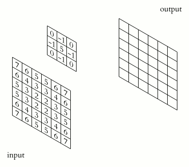
The convolutional Layer (CONV)
The most computation in the ConvNet is made in the convolutional Layer. It holds the weights and biases as input Paramters of our model and uses them to calculate the output
in a remarkable way.
The convolutional Layer consists of N learnable spatial filters of size $(F \times F \times$ Depth of input$)$ stacked along the depth dimension putting out a Layer of
final size $(F\times F \times N)$. The 2-dimensional $(F\times F)$ output of one filter is called depth-slice. So we put in every depth-slice a certain amount of neurons.
The neurons take the filter of the depth slice they are set in as retinas and convolve locally their weights with the input data they can see. During the computation we slide
the filter across the width and height of the input volume and let the neurons locally convolve their weights with the input data they can see because of the filter.
Take care that after every convolution the result is added with the bias of the corresponding neuron.
Michael Plotke, CC BY-SA 3.0, via Wikimedia Commons
Why are we restricting the input of the neurons by the Filter? Think about a picture of an car on the road. The spatial extension of the car on the picture
is restricted to some amount of pixels since the car isn't covering the whole picture. By thinking that in general our model wants to classify the object on a abitrary road as a
car it should not take the background too much into account while analyzing the pixels of the object on the road since we aren't interested in the background.
For example if our car is driving on some mountainious landscape the pixels of the mountains on the background are not helpful to analyze the object on the road.
To implement this in our model we introduce the Filters and restrict the retinas of our neruons. This implementation also reduces the amount of parameters we need to introduce,
thus reduces overfitting.
Suppose our input data has the given volume of size $(W_1 \times H_1 \times D_1)$. Then the CONV Layer produces a volume of size $(W_2 \times H_2 \times D_2)$, where variables
can be determined by the following formulas.
\[
W_2 = \frac{W_1-F+2P}{S} +1
\]
\[
H_2 = \frac{H_1-F+2P}{S} +1
\]
\[
D_2 = K
\]
There are Some parameters used that weren't introduced yet. These are called Hyperparameters and
they are useful to control some properties of the CONV layer and the model in general.
\[ \]
-The number of filters used in one CONV layer : $K$
\[ \]
-The spatial extend of the filters filter size or the receptive field of the neurons (width,height): $F$
\[ \]
-The Stride: $S$
\[ \]
-The amount of zero padding: $P$
\[ \]
-The Filter size F controls the connectivity of the neurons to the input data while convolving. In classical neural nets the neurons are fully-connected to
the input data which causes overfitting since the amount of parameters for fully connected layers grows fast. So threshholding the neurons to some data region reduces the
amount of parameters needed and thus is an laverage for overfitting.
\[ \]
- The Stride S is used to control the number of pixels the filter moves at a time in both directions width and height. This influences the output volume in the
the mentioned two dimensions.
\[ \]
- Zero padding P puts zeros around the border of the input volume in amount of P. This is implemented to use filter sizes which normally wouldn't fit on the
input data. This can be easily seen by the formulas of W2 and H2 above. Notice that these two numbers have to be intergers since the Layers of a ConvNet are volumes made up
of a discrete amount of neurons and that for a given input volume, Stride and a zero padding of zero not every filter size fits this condition.
\[ \]
How many neurons do fit in one depth slice of the CONV Layer ? \[ \]
Well this is easy to answer since we know the widht and height of the depth slice in relationship to the input volume.
So the number of neurons $N$ in one depth slice is
\[
N = W_2 \cdot H_2
\]
In total There are $N*K$ neurons in one CONV Layer. Now important is, how many parameters does one CONV layer need for a given input
and Hyperparameters. Every depth slices needs $N\cdot F \cdot F$ weights and $N$ biases. This is in Total $(N \cdot F \cdot F \cdot D_1+N) \cdot K$ parameters. This amount of parameters
are to much thus causing overfitting. One way to reduce the amount of parameters is called paramter sharing. In this case all neurons in one depth slice share the same weights
and bias. This simplification leads to a amount of $F\cdot F \cdot D_1 \cdot K + K$ parameters in total.
For example training our model on MNIST pictures we will use a Filtersize of $F=3$, a stride of $S=1$, a Padding of $P=0$ and $K=32$ filters for the first (CONV) layer.
Our input data will have a volume of $(28,28,1)$ and thus the first (CONV) layer spits out a volume of $(26,26,32)$. The number of Neurons in each depth slice is then
$N=26*26=676$ and without parameter sharing we would need 6760*32=216.320 Parameters for just one (CONV) layer. With parameter sharing this amount reduces to 320 Parameters.
So we see that parameter sharing drastically reduces the amount of parameters needed.
Note: Overfitting happens when your model fits your training data well, but it isn't able to make accurate predicitons for data it hasn't seen during training.
the pooling Layer (POOL) and the dropout Layer (DROP)
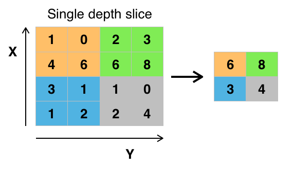
The function of the pooling layer is to progressively reduce the size of the input volume to reduce the amount of parameters and computation in the network.
The pooling Layer operates independently on every depth slice of the input and resizes it using the MAX operation. For the POOL layer we need to introduce one filter of
dimension $(Width \times Height)$ which the neurons take as retina, but this time no convolution with their weights happen instead they use the MAX operation to always take
the biggest value of the inputs they can see. During the computation we slide the filter across the width and height of the depth slices independently let the neurons locally
use the MAX operation.
Note: Since the neurons don't engage with the input Data via convolution there are no parameters needed in this case. So the layer posseses no input parameters.
Suppose our input data has the given volume of size $(W_3\times H_3\times D_3)$. Then the CONV Layer produces a volume of size $(W_4 \times H_4\times D_4)$,
where variables can be determined by the following formulas.
\[
W_4 = \frac{W_3-O}{S} +1
\]
\[
H_4 = \frac{H_3-O}{S} +1
\]
\[
D_4 = D_3
\]
The Hyperparameters of the POOL layer are:
\[ \]
-The spatial extend of the filters filter size or the receptive field of the neurons (width,height): $O$
\[ \]
-The Stride: $S$
\[ \]
The common filter Size O and Stride S of a POOL layer is O=2, S=2. This discards 75 percent of the activations (inputs). One needs to be careful with the Filter Size F since
too large receptive fields are too destructive.
Aphex34, CC BY-SA 4.0, via Wikimedia Commons
The Droput layer (DROP) disables a certain amount of neurons in the input layer for the next calculations in the ConvNet. So after passing the DROP layer
some of our input for the following layer will be disabled meaning that the neurons in the follwing layer can't see the output of these disabled neurons.
This happens randomly and is controlled by a hyperparameter $Q$ which ranges from 0 to 1 dropout. So with a probability of Q the neuron is staying active for the next calculation
and with a probability Q-1 it's going to be disabled.
The fully-connected Layer or dense Layer (FC)
Neurons in a fully connected layer have full connections to all activations in the previous layer. This layer is used as last layer of the ConvNet to extract class scores and
thus in thiscase refers then to the output of the ConvNet. The volume could have a shape of $(1 \times 1 \times$Number of Classes$)$. Note that in this layer the neurons convolve
their weights with all the input data for one time.So the filtersize is as big to fit on the input data for one time.
Note: This layer posseses weights, which will be trained during the training process and there's no parameter sharing existing.
The activation function layer; E.g. the RELU layer (RELU)
The activation of the neurons are separated into one layer of the network. There are several activation functions that can be used to fire the neurons in our case we will use the rectified linear unit (RELU) activation function for the activation layer. The RELU layer takes the input volume and uses the activation function on every discrete element of the Volume while remaining its volume unchanged.
How to order these layers in the network
One way of ordering the layers in a ConvNet could be
\[
INPUT->CONV->RELU->POOL->FC->RELU->FC.
\]
Notice that the last FC layer is considered to be the output. Here we used only one CONV layer, pooled the output, fully connect them, let the neurons fire again with RELU
and lastly get the output. There are several ways to stack the layers.E.g. we could use two CONV layers
\[
INPUT->(CONV->RELU)\cdot 2->CONV->RELU->POOL->FC.
\]
In our case the neurons in the CONV layer always fire with the activation function RELU right after the convolution.
Note: Keep in mind that the last layer corresponds to the output of the convNet and thus should have an appropriate size to describe a class score.
Why do we care about overfitting
The purpose of machine learning modells like the ConvNet is to generalize. By this we mean the abillity of the model to give useful outputs to input Data it has never trained on before. If this is the case our model successfully catched all the for generalization reliable structures of the training data, which minimize the calculated loss and are capeable to predict the new input Data. But also while training the model can possibly recognize some secondary structures of the training Data and try to lower the loss even more by also noting them. Eventhough learning these secondary structures lowers the loss, our model now took information into account which are uniqe properties of the training Data,called noise. This information isn't useful for generalization and thus hinders the model to be more efficient. In this terms overfitting means that the model catches the noise of the training Data.
The Loss function
The loss function is a measure of how good our deep learning algorithm predicts the rigth classes for the the data. Its a scalar value which we want to be as low as possbile.
As mentioned the score function consumes all our data and gives out for every Data a column vector $\vec{s}$ representing the class score. Note that every row in the column
vector stands for some class. The values in the class score are abstract numbers which we can interpret as "probablities" $p_i$ that the $s_i$-th class is the right one
if we act on them with the softmax function.It takes an N-dimensional vector of real numbers and spits out a N-dimensional vector $\vec{p}$ with entries in range between 0
and 1.These "probabilities", entries of $\vec{p}$, are given by
\[
p_i = \frac{exp(s_i)}{\sum_{k}(exp(s_k))}.
\]
Note that if we sum over all $p_i$ we get one and thus a correct normalization.
\[ \]
How does this help us to implement a loss function?.
Now that our modified scroe function gives out a predicted probability distribution $\vec{p}$ and in addtion we also know the right class distribution $\vec{s_r}$ we can go
one step further and define the cross entropy between these distributions and use this expression as our loss function. Note that the $\vec{s_r}$ column vector consists of
entries of zero except for the right class, where the entry is one.
The cross entropy for the prediction of one data $x_n$ is defined as
\[
H (\vec{s_r},\vec{p})_n=- \sum_{j}({s_r}_j*log(p_j))=-log(p_n),
\]
where the entry $p_n$ of the vector $\vec{p}$ corresponds to the true class of the data $x_l$ and this is considered to be the loss of the data $x_l$.
Note that for probability $p_l \to 1$ our loss gets zero and for probability $p_l \to 0$ our loss gets infinity and thus gives plausible values. Now the loss
function for the whole data-set is
\[
L_{m} = \frac{\sum_{l}H(s_r,s_p)_l}{M},
\]
where M is the amount of our data and the sum goes over all our data.
Note: The reason I put "probabilities" in quotes is that these quantities depend on some regularization parameter lambda which constrains the weights we use in the convNet.
The change of lambda can cause a diffusion in the values of the probablitiy distribution and thus influences how peaky the distribution is. For this reason we should talk about
confidences and not probabilities.
The training of the ConvNet
the question that comes up now is that how do we train our deep learning algorithm to predict proablitiy distributions peaky enough on the right class to make correct predicitions.
As mentioned in the begining chapters we do this by minimizing our loss function in dependency of our weights W, which are our input parameters. So we continiously update our
weights to a desired value $W_{min}$ where our loss function spits out the value of an local minimum. Note that by the predicted class scores $\vec{p}$ our loss function depends
on the weights and biases.$L=L(W,b)$.How exactly is this done? Imagine you were put randomly on a place of a uneven surface and
you want to find a local minimal spot on the surface blindfolded. The strategy could be to scan the surface with your foot and make steps along the direction wehere you feel a
negative slope. You would also need to consider how big your step should be since the extension of the mininal spot is finite or your don't know how far it goes down.
To put our case in analogy we start the computation of our scores with randomly initialized weights $W_{init}$. Then we calculate the loss that these weights cause
to find our starting spot. Now to know in which
direction we should update our randomly initialized weights we basically need to calculate the gradient of the loss function with respect to our weights. From diffierntial
geometry we know that the gradient of a function points in the direction of the steepest ascent. So going to the opposite direction of the gradient is the steeptest descent
and updating our weights in this direction will cause the loss function to decrease. While taking the analogy we need to be careful since our loss function lives in a high
dimensional space far away from the intuitive three dimensional space. To be precise the vector space in which the loss function lives has as many dimensions as we put
parameters in our network. This method is called Gradient Descent.In mathematical terms the Gradient Descent looks like.
\[
W_{upd} = W_{init} - r \cdot \nabla_WL
\]
Gradient evaluated at $W=W_{init}$.
In general the i-th update looks like
\[
W_i = W_{i-1} -r \cdot \nabla_W L
\]
Gradient evaluated at $W=W_{i-1}$.
So the updated Weights $W_{upd}$ are updated in dependency of the step size $r$ also called learning rate. This Hyperparameter controls
how far we step along the steepest descent of the loss function. Taking small steps assures consistent but very small progess while taking large steps leads to a faster
descent but as mentioned in the analogy the extension area of the minimal spot is finte. So taking a big step could cause that you get off the desired direction and actually
take a step in direction of the highest ascent.Thus the parameter update would cause a increase of the loss function and with this no convergence of the loss happens.
But if your stepsize is to small it could cause you to
stop before reaching the minimum while training. So there's also a risk in taking a too small stepsize. There exists more ways to train the convNet which I will not describe.
Note:Calculating the gradient of the loss with respect to the weights of the neurons is called backpropagation. So the gradient of one neurons weights is considered to
be the feedback it gives back to the system as whole.
Training a ConvNet with MNIST
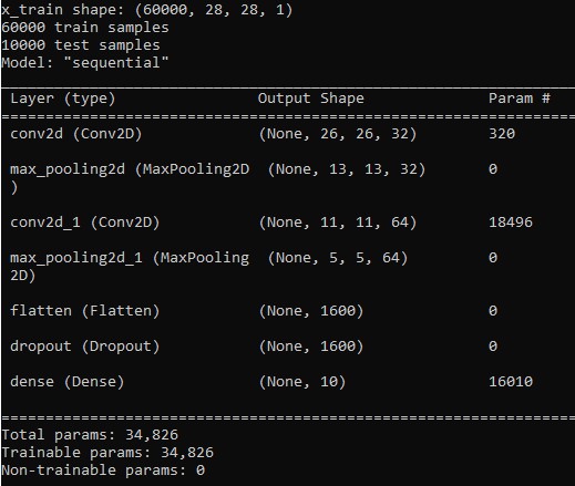
In the following we got a Dataset (MNIST) of 70,000 pictures of handwritten Digits between 0 and 9. Thus we got 10 classes. We will take 60,000 pictures of the Dataset to train our ConvNet and after the training is complete we will test the validity of the predicitions of our ConvNet on the remaining 10,000 Data. the pictures of MNIST are made up of 28 pixels along width and height and posses one color channel, which is needed to represent pictures in black and white. Thus the depth of the pictures will be one. So the input volume of our ConvNet will be of size (28x28x1). The platform used to train the convNet will be phython where we use Tensorflows deep learning API keras. On this plattform the volume layers will be saved as arrays and all the computation will be done with this instance. The following picture shows the strucutre of the network we use. It also shows the params that every layer holds. With the formulas in the previous sections one can sanity ceck the number of params the CONV layer has to hold.
We will use here a sequential model of Keras. The model trains by splitting up the training data into batches.It takes the first batch, calculates the loss and the accuracy and then updates the weights with the Gradient Descent method.The updated ConvNet takes then the next batch and repeats the steps. At the end we see the loss and accuracy after the model went through the last batch of the training data.One such passing of the ConvNet of the training data is called epoch. Usually we will train our ConvNet for several epochs, in our case $10$ Epochs. To find out if the convNet is overfitting we introduce the cross-validation technique. So before splitting our data into training batches we take a certain percentage of the training data aside and call this data validation set. The validation set is only used to evaluate the performance of the convNet after every epoch.Therefore after every epoch in addtion to the loss and accuracy (acc) of the model on the trained data we will also get values, val_loss and val_acc, calculated on the validation set. These quantities are calculated after the last update in one epoch. Now if acc is higher then val_acc then this a hint for overfitting. In our case the size ofthe validation data will be 10 percent of the input Data, which we adjusted so.
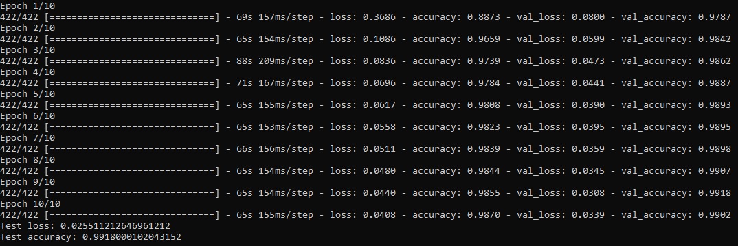
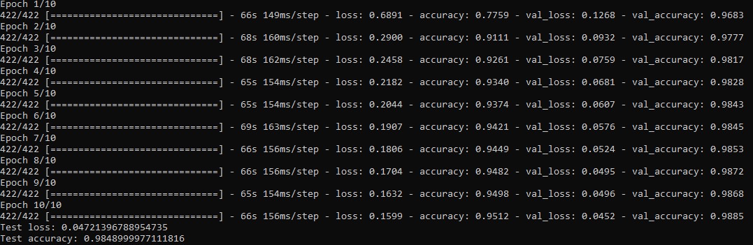
Picture2 shows the training history of our Model training for $10$ Epochs with a Batchsize of 128 datas. We got $60000$ data units and take out $6000$ for our validation set.
The remaining data is sliced into $422$ batches of sice $128$, its actually $421,875$ but we have to round up thus the last batch has actually less than $128$ Data units inside.
The first value in units of seconds shows the training time in one Epoch. The second second value shows the training time per batch.We can see that for the Epochs in the
beginning the loss decreases and the accuracy increases in both Datasets,training and validation Data. We also see that for these Epochs the accuracy of the training Data is
smaller than the validation Data accuracy meaning that our model isn't overfitting. Remarkable is that in the last Epoch, Epoch = $10$, our validation Data loss increases and
validation accuracy decreases, while on the training data wee see a reverse behavior.This means that our model starts overfitting thus we should stop the training after Epoch=$9$.
This could also be some fluctuation so to determine the reason we should train the model for some more Epochs and compare the metrics.
The last two values at the bottom of picutre2 we see the loss and accuracy calculated on the test set of $10000$ images. Our trained Convolutional Neural Network predicts
with a probability of over $99$ percent the right label of the test picture.
In the following I will change some parameters of this model and discuss the change of our metrics and calculation time while training.
Changing the learning rate r
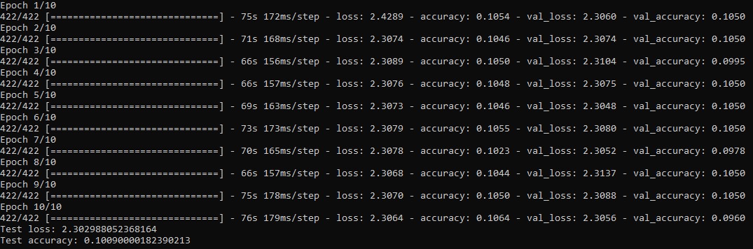
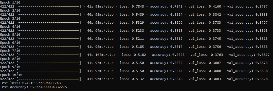
Picture3 shows a training history where the learing rate is increased to $r=0.1$. We can see that theres no significant change in the calculation time. The more interesting part is the loss and accuracy of our model with this learning rate. As mentioned bigger learning rates lead to a faster progress while risking a lack of convergence. This can can be seen here. The loss halted at some high spot and alternates by a small amount between the different Epochs. Thus our model only reaches an accuracy of 10 percent on the test set.
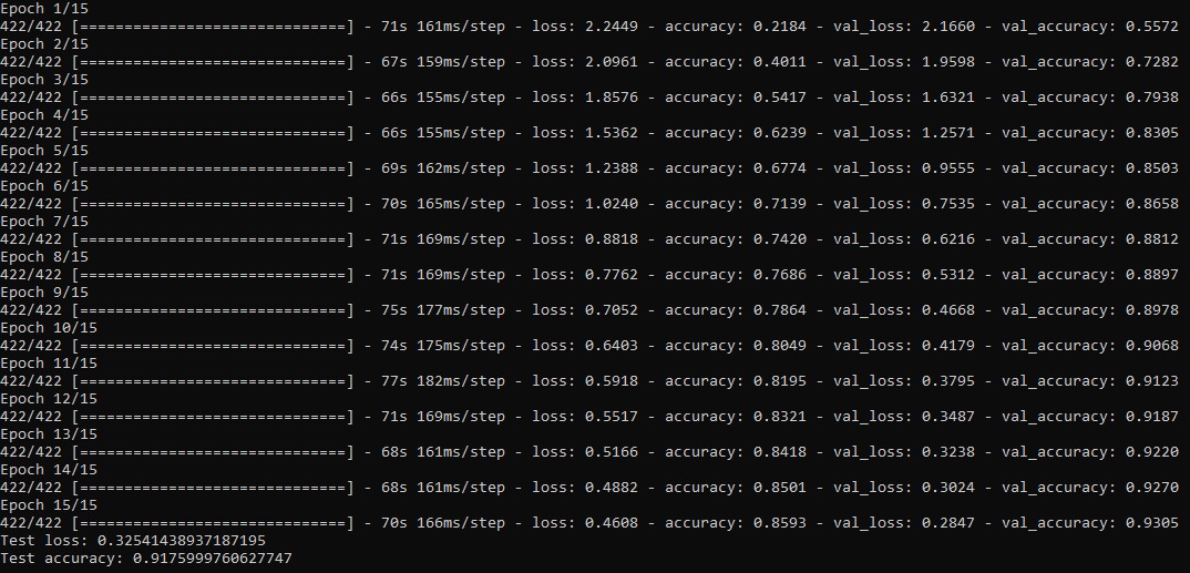
Picture4 shows a training history where the learning rate is increased to $r=0.00001$.Again we can see thath theres no significant change in the calculation time but a different behaviour in the progress of the loss and accuracy in the model. Here we can see the discussed slow convergence very clearly. Eventhough we extended the Epoch size to 15 the model still didn't reach the accuracy of our model in default with 10 Epochs. Also important to realize is that the model converges to some value which wasn't given in the previous change of the learning rate.
Changing the dropout Q
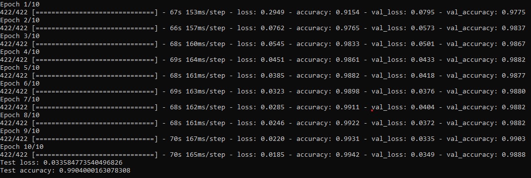
Changing the dropout to $Q=0.01$ leads to a different behaviour, which is more subtle. Looking at the metrics of the Epochs we can see thath the accuracy of the traing gets slightly larger than the accuracy of the validation set. The turning point is Epoch 5 and by this we see that the model predicts its trainig data (old) better then the validation data (new). Our model losses it's abillity of generalization to new data which we want to avoid.
In Picture6 we can see that setting the dropout Q to high the model gets to less information to work fast. Thus the it needs more time to train to reach the accuracy of the model in default mode, Picture1.
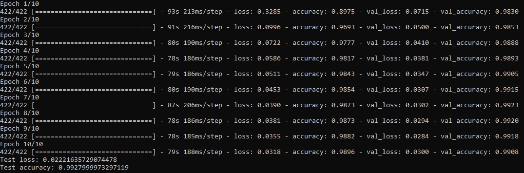
Changing the filtersize F
Increasing the filtersize of Kernel in the Convolutional layer to $F=5$ leads to a larger calculation time but only a slightly change in the metrics of the training. The model converges sligthly faster with the increased filtersize. So its reasonable to reduce the filtersize of the Kernel to $F=3$ to minimalize the training time.
Decreasing the filtersize to $F=1$ leads to a smaller calculation time but the metrics of the model needs some time to converge. While training for 10 Epochs the model reaches a significantly smaller accuracy than the default model. So its reasonable to increase the filtersize of the Kernel to $F=3$ to converge faster.
Summary
Deep learning with a convolutional neural network is useful to classify pictures. Using methods like parameter sharing, dropout or dooling we introduced some leverages to decrease the distraction of overfitting and make it possible to get reliable results. These kind of methods are regarded as regularization tools and there exists more of these we didn't discuss here. In general the true challenge is to find the right combinations of Hyperparameters for our model to make it as general as possible.
Source
[1] https://cs231n.github.io/
Note: These are the lecture notes of a visual recognition course of the Stanford University.