Simulation environment
The simulation consists of simple cars on a roundabout. The Roundabout has one lane, so the cars follow each other in a constant order. The cars are build out of a box, which represents the body of the car, and four cylinders, which represent the wheels (Figure 1, left). The two front wheels have motors. Each car has a radar, which represents the sight of a driver. The radar frustum is shown in Figure 1, right with the blue lines. A car has information about the car in front only when it is inside its sight.
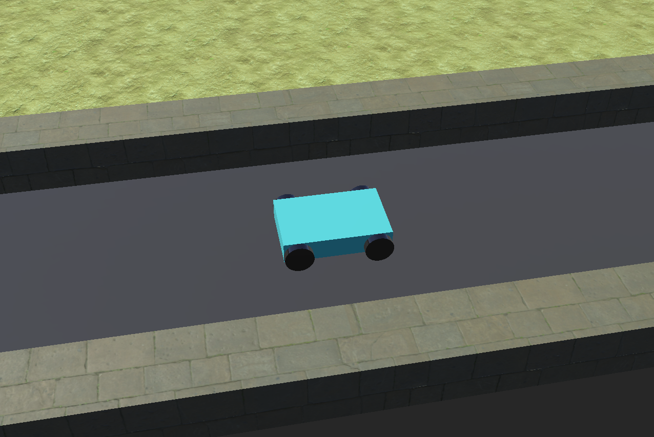
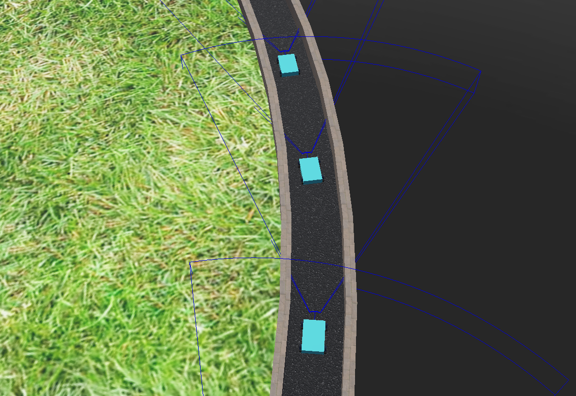
Figure 1: left; Simple car on the road. right; The blue lines are representing the radar frustums.
Simple linear model
In the simplest model a car's acceleration only has a linear dependency on his velocity relative to the car in front.
\[ \ddot{x}_{j+1}(t+T)=\lambda\cdot[\dot{x}_{j}(t)-\dot{x}_{j+1}(t)] \]The proportionality constant $\lambda$ it the reaction strength of the drivers, and $T$ is the delay in the reaction. In the numeric simulation, the radar gives the distance to the next car each time step. The change in distance from the previous time step to the current one is the relative velocity. Multiplying the relativ velocity with $\lambda$ gives us the change of the velocity for the time step. This change in velocity is then the update for the next time step. In each of the simulations shown here, $\lambda$ is adapted to the system, so that the motions remain stable.
The first car in the line maintains a constant velocity when there is no added perturbation. This case is shown in the left video below. In the video on the right, the first car's velocity preturbes, oscillating around a constant value. In this videos there is no time delay, so $T=0$.
Neglecting the small perturbations caused by the curvature of the roundabout, the relative motion of the cars in the video on the left remains constant. In the video on the right, the oscillations of the first car cause congestions. The cars sometimes bump each other, since they can't slow down fast enough, because in this model the acceleration depends only on the relative velocity, not on the relative distance.
In theory, adding a time delay should cause congestions that oscillate from the front of the line to the back. This is tested in the next two videos below. On the left, the time delay is an order of magnitude smaller then the perioud of oscillation of the first car. On the right, the time delay is still smaller then the oscillation of the first car, but in the same order of magnitude.
Some time is needed for the perturbation to show it's effect, but then both videos show congestions that move along the line of cars. In the video on the right where the time delay is bigger, the congestions have a larger wavelength, so they are more clearly visilbe.
Non-linear model
\[ \ddot{x}_{j+1}(t+T)=\lambda\cdot\frac{\dot{x}_{j}(t)-\dot{x}_{j+1}(t)}{{[x_{j}(t)-x_{j+1}(t)]}^{1+\alpha}} \] In this model a non-linear distance dependency is added. In the simulations here, $\alpha$ was set to 1, so the distance dependency was quadratic. This is a more realistic model. It can be seen in the simulations that the cars don't bump each other. They slow down quick enough. Below in the video on the left the the model is tested without a time delay. On the right, a time delay is added. As before, $\lambda$ was adjusted, so that the movement remains stable.
After some time, both videos show congestions propagating from the front car to the back. With the time delay the wavelength of the concestion is bigger, since there is only one in the video on the right. Such traffic developement occures in real life, so this model gives a good picture of a part of everyday traffic.
At the end, another simulation is shown, in the video below. Now both the reaction constant $\lambda$ and the time delay $T$ are increesed. This is an example of a crash that happens because the drivers react late and strong. The chras happens at the top of the roundabout, in the ending part of the car line. By watching closely, on can see that some cars even start to drive backwarts. That is because $\lambda$ is too high.