Description
The goal of this project is to program a self-learning robot which is able to teach itself how to walk. Doing this should not include hardcoding of any movements, but instead rely on a neural network controlling the motors. An artificial evolution algorithm finds the most efficient configuration of the network using a supervised learning technique.
Interesting results could be:
- The underlying connection between the movements of different motors.
- How the Fitness of the population changes over time depending on the starting parameters.
- How the robot chooses to walk.
The network uses two neurons to calculate the motor signals from given inputs. Every network in a generation is being tested before a new generation is bred. As a measurement of Fitness we used the distance the robot traveled in a set time interval. Below you find videos showing the evolution of the robot, more details about the controller and plots and interpretations answering the questions above.
Footage and Results
An Example Run
Let us now take a look at a run with a population of 50 and a total of 50 generations. We will not only show the state of the robots at several points but also discuss emergent behaviors and patterns. All videos are created using a program called simple screen recorder, for the plots we used gnuplot.
Generation 1
You can click on all images to enlarge them.


Here you can see three robots being controlled by three different networks with randomly initialized weights. These are representing the first generation. Below them you find three plots showing the motor commands given to the robot by the network at any given time. We will concentrate on the rear legs as they are the main force driving the robot forward. The flat bits indicate that the network "maxed out" the sigmoid function we used as an activation function. The x-axis shows the time in simulation steps. Note that all three robots have quite random commands to work with.
Generation 5

The video above shows the best robot at the end of generation 5. Looking at the plot, one can see the commands for the right rear hip and knee have a phase difference of pi, making the robot move its right hip back while moving its left leg forward.
Generation 10

Generation 15

We have now reached generation 15, the system has developed a not-so-smooth but quite effective walking pattern, which is apparent in the plot.
Generation 25

For generation 25 the robot not only manages to get much further than before, looking at the plot one can even see the system "choosing" a simpler and far more effective motion sequence. From now on the best networks will "try" to make big and fast steps to get as far as possible in the given time interval. There are no short pauses anymore and the movements of both legs are almost perfectly in phase.
Generation 50

This last video shows the final result of the run. At generation 50 the robot is not improving anymore as you can see in the first plot on the right showing the highest Fitness of each generation (details about the Fitness function can be found in the next section). The plot next to that shows the average Fitness of each generation. The commands plot shows that the controller has found a very stable solution by moving the legs as quickly as possible from one side to the other. There is not a lot of room for further improvements.
Looking back at the plot showing the Fitness over time one can clearly see the benefit of using artificial evolution, as the system finds a stable solution quite fast. It will take time to optimize the solution, but it solves the underlying problem quickly.

Parameters
The last part of this section will focus at some of the parameters available to us (we will not show any videos as the results look the same as above):
- Chance of mutation m
- Number of networks per generation n
- Type of Fitness function f(x)
Chance of mutation m

m = 1

m = 0.5

m = 0.25

m = 0.1

m = 0
As a first step we will determine the role of mutation (see the section details for further information). From left to right you can see the highest and average Fitness using different values for m. Every other value stays unchanged compared to the example run above, which used a value of m=0.05. Note that the y-axis now has a smaller scale compared to the example above.
You can immediately see how great a role mutation plays. A value of one causes the weights to be completely random in each generation, meaning we will never become better than any of the networks of the first generation. Even with m=0.5 the Fitness stays extremely low (the small spikes are due to random fluctuations). At m=0.25 we observe an interesting behaviour as the curve spikes quite high for certain generations. On the other hand, if we take a look at the average Fitness we do not see any difference. Apparently a value of m=0.25 seems to hit some kind of a sweet spot, even if we do not get an overall learning effect. A value of m=0.1 shows mostly the same result as m=0.25, with the exception of there being no spikes. The randomness still hinders any fast learning, we do get a smoother curve though.
Of great interest is m=0, as it shows that zero mutation is not the way to go either. Compared to the other plots it shows greater success but the robot stops to learn at some point. All networks are the same after reaching generation 40.
Number of networks n

n = 10

n = 25

n = 100

n = 250
Back at m=0.05 we want to investigate the importance of the population size. We compare sizes by testing a total of 2500 networks (as in the examples above: 50 networks per generation, 50 generations).
The first plot shows that choosing too small of a population size will reduce the systems learning rate significantly. There is just not enough variation available. The next two plots for n=25 and n=100 look very similar to the result of the example run while n=250 shows a significant drop off. Apparently the other extreme hinders the learning process as well as there is too much variation and the "breeding process" is too random (you can clearly see that n=25 is at a much higher Fitness level than n=250 prior to generation 10).
Type of Fitness function f(x)

f(x) = x

f(x) = sqrt(x)

f(x) = exp(x*x)

f(x) = x²
To compare different functions to each other we used the standard Fitness function for the plot and the new one internally to "breed" the networks together. Apparently all of them are less suitable compared to the one we used in the example. Only with the x² one we were able to reproduce an even remotely similar result. Lets now look at each of them individually.
The reason the Fitness is so low for the linear case is probably the small difference in Fitness for each network. Especially in higher generations the breeding algorithm is still taking networks with a much lower distance into account. The sqrt one has a similar problem, as it is quite steep at lower distances, but becomes very flat for increasing distances, so the difference between two similar networks is large at the beginning but small for later generations (with higher average distance achieved). The opposite of the linear case is the exp(x²). There is an enormous difference between similar networks resulting in a very high chance to breed with the same few networks, namely the ones with the highest Fitness. This circumstance hinders the process of generating better networks through including different "genes". The x² case seems to be appropriate as we have small differences between networks with smaller distances and larger between networks which achieve slightly higher distances.
Details
Below you can find a more detailed description of the robot, as well as network and controller.
The robot
For the project we used one of the prebuild robots included in the LpzRobots download. It is called "vierbeiner". The code itself was kept mostly intact, with the only notable change being the addition of three extra sensors used to measure the position in order to calculate the Fitness of a given network. The robot has 10 motors for the legs (two at each front leg and three for each at the rear).
The network
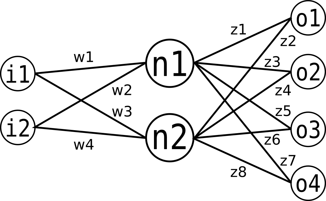
The self-made network used is a single layered neural network with non-timedependent weights. All inputs are connected to the layer of neurons which are in turn connected to the outputs. As an activation function we used the sigmoid function
where x is the sum of all inputs multiplied with the respective weights of the synapse. An important point is that the networks outputs lie between 0 and 1. The input values propagate through the network as follows (here we use the image above as an example, the actual number of nodes may vary):
To calculate the values for each neuron we multiply the input (as a column vector) with the matrix containing the first four weights (w1 through w4):
Applying the sigmoid function to n1 and n2 and multiplying the resulting column vector with the matrix for the eight weights z1 through z8 results in the output vector:
The last step is to apply the sigmoid function once more to the output vector.
The controller
As a basis for our controller we used the "walkcontroller" included with the vierbeiner-robot. Here we connected the controller with the neural network giving it two time-dependant inputs with a parameter s changing the speed and a parameter v changing the strength of the input. Increasing the speed by reducing s will result in faster movements of the robot, changing v modifies how strongly the network reacts to input changes.
We found that giving the network more inputs (one could assume that one input per leg would be optimal) made the result more chaotic instead of improving it. The output of the network is directly put back into the simulation as the motor commands for the robot.
Genetic Algorithm
As a mean to improve networks jumping from one generation to the next we used a genetic algorithm. It can be summarized as follows:
SETUP:
- Step 1: Initialize. Create a population of N elements, each with randomly generated DNA (weights on the synapses).
LOOP:
- Step 2: Selection. Evaluate the fitness of each element of the population and build a mating pool.
- Step 3: Reproduction. Repeat N times:
- Pick two parents with probability according to relative fitness.
- Crossover - create a “child” by combining the DNA of these two parents.
- Mutation - mutate the child’s DNA based on a given probability.
- Add the new child to a new population.
- Step 4. Replace the old population with the new population and return to Step 2.
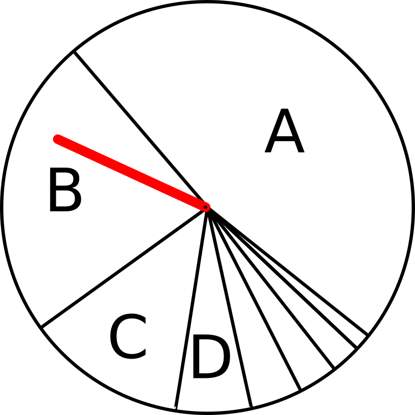 The networks are chosen by taking their Fitness into account. Network A has almost twice the fitness than network B.
 Network A and B are combined to form the new network C. After this network C will be mutated.
 The generation N' is being bred using two networks of generation N for each new network.
At the beginning of the simulation the controller initializes the first generation, which size can be manually set, with random weights on the synapses (Step 1). When the simulation starts, the first network is used to control the robot and its Fitness is measured (Step 2). After some arbitrary time (we chose 500 simulation steps) the controller switches to the next network and the process starts again until all networks of one generation are tested.
The Fitness function we used is
with d being the distance in the direction of the x-axis (forward).
After a generation has finished two networks are chosen, using the Fitness value as a means to weighten the probability to use the network to "breed" a new network (Step 3.1). During this "breeding process" the weights of the "parents" form the new weights with a chance of 50% to use the weight of one network over the other (Step 3.2). After this process of combining the weights of both "parent" networks the weights are mutated, changed with a very small probability (Step 3.3). As each breeding-process only produces one new network, the algorithm chooses N Network pairs to form new networks. This process will repeat until a completely new population is "bred", then the whole process starts over again (Step 4).
Acknowledgements, Authors and Contact
- Acknowledgement We would like to thank the members of the group Prof. C. Gros, especially Laura Martin and Hendrik Wernecke, for their help developing this project.
- About the authors Lars Gröber and Philipp Arnold are both Bachelor's students at Goethe University Frankfurt (Main).
- For questions, suggestions and comments please contact lars.groeber@stud.uni-frankfurt.de.
Download and References
As references we used the following material:
- The Nature Of Code by Daniel Shiffman
- Wikipedia article about genetic algorithms
- Videoseries about neural networks.
Here you can download the project files.
The project uses the LpzRobots-package developed by the University of Leipzig. An additional dependency is the Armadillo-package which needs to be installed.
- The actual robot is configured in
vierbeiner.*. - The controller is configured in
walkcontroller.* class.simpleNeuralNetwork.hcontains the network class.
- Move the files into the folder
YOUR-LPZROBOTS-DIRECTORY/ode-robots/simulation/. - Execute
make && ./startinside the folder "vierbeiner-robot". - While running the program will
- print to the console the current network/generation and its Fitness/highest Fitness.
- write the highest and average Fitness into a file called
fitnessin the formatgeneration highest-fitness average-fitness. - write the motorcommands of the best network after each generation into a file called
motorData/motorOutput#(where "#" stands for the current generation). - use at the end of the last generation the best network.