Analysis of Swarm Behaviour and Flocking Phenomena
Self Organizing Simulation using the LPZ-Robots Package
Abstract
Inspired by many phenomena in nature, like the swarm behaviour of the starling, we studied self-organized flocking effects of a swarm of two-wheeled robots, using the LPZRobots environment.
Basically, the idea was to implement one leading robot which prefers to travel in one direction, only avoiding collisions with obstacles along its way. A predefined number of other robots is supposed to create a typical swarm behavior by aligning the own velocity to the velocity of the closest neighbours.
This model allowed to scetch the flocking behaviour of the swarm for different parameters, e.g. the interaction length of the robots and the density of obstacles in the field. It could be observed that the number and size of the swarms differ drastically for different parameters. Also the number of robots travelling in the definite direction of the leader is very sensitive to changes of these parameters.
Model & Theory

Fig 1.1: The robot we used for our swarm analysis
For our Analysis, we modelled a bird flock by using the two-wheeled robots, already defined in the LPZ-Robots package. For obstacle avoidance, we equipped every robot with further IR (Infrared) - sensors, that can influence the motor's power setings in order to turn the robot away from any object in it's way. In addition, each robot carries as many RelativePositionSensors, as robots were generated in the swarm. These sensors give the current position of the corresponding other robot in relation to the carrying robot.
Code

Fig 2.1: The basic structure of our code
- Zip-File containing all relevant files
The files originate from the LPZ-Robots Package, as stated under Sources.
We have engineered the files with the greatest possible care, tested them multiple times and are confident that they should run flawlessly.
We do however not take any form of liability for any damage to your hard- or software that may arise from the use of these files or any affiliated software.
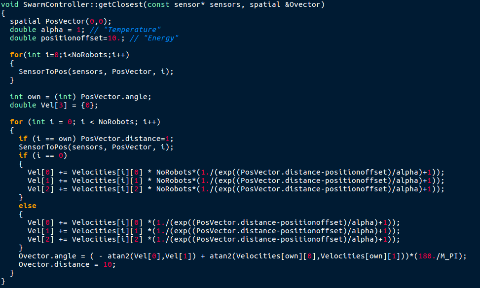
swarmcontroller.cpp GetClosest()
The function 'getClosest()' changes the value of a given double. First, the function SensorToPos is called (see below).Then, the group velocity vector is calculated. For that, all robot-velocities are added together with a weighting funciton, the Fermi distribution. The leading robots velocity has a higher weight, otherwise it would not matter at all.
Finally the angle between the target velocity and the robots own velocity is calculated and written over the given doublt.
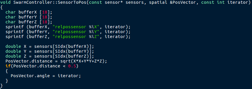
swarmcontroller.cpp SensorToPos()
SensorToPos reads the relativepositionsensor to another robot. It changes the spatial 'PosVector':PosVector.angle contains the number of the current robot (it is only changed if the distance is very small, so it has to be called for all robots in order to actually obtain the robots number).
PosVector.distance contains the distance between the current robot and the given robot.
swarmcontroller.cpp VelSetter
VelSetter sets the member variable velocities of SwarmController. The function gets called in main.cpp.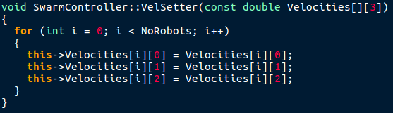
swarmcontroller.cpp Motorcontrol
This piece of code controls the motors of the swarm robots. If there is an obstacle in front of the robot, go back, if there is an obstacle on the left side go right, if there is an obstacle on the right side go left. Since the left IR sensors are called fist, the swarm tends to go to the right if the obstacles are directly ahead. The 'Swarm' part of the movement comes from the else and is also regulated with a Fermi distribution for extra smoothness.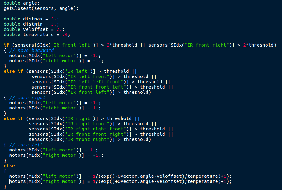
main.cpp start()
In the start function in the main.cpp file the we had to store the pointers to the robots in order to set the RelativePositionSensors later. We stored them all in an array and set the references for the RelativePositionSensor later (see the last for loop in this code). The initial position of the Robots is set in a square of arbitrary size.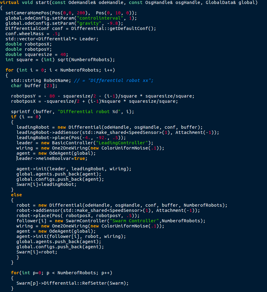
Results
Video 1: Behavior of a robot swarm when no obstacles are present
Video 2: Behavior of a robot swarm when confronted with a low obstacle density
(2% coverage)
Video 3: Behavior of a robot swarm when confronted with a high obstacle density
(10% coverage)
When no obstacles are placed in the playground, the robots follow a tight swarm only disturbed by minor noise in the sensor readouts.
When a few obstacbles (2% coverage) are placed in the playground, the robots soon begin to split into several smaller flocks that can recombine when they come close enough to each other.
When many obstacbles (10% coverage) are placed in the playground, the robots directly break up into many very small flocks or single robots, resulting in a chaos-like distribution.
Analysis
In the following section, we will present a series of data sets. For every line, we have varied certain parameters, as can be seen in the table.
The first plot shows the angular orientation of every robot's velocity versus the time. Hence a coherent swarm will produce a straight line, while a scattered crowd will result in a broader distribution.
The top right graph is the corresponding Fermi-distribution function, that was used for the correlation of the robots in the simulation run.
The last image on the bottom right depicts a scheme of the obstacle density on the playground. Note: It is not the actual distribution that was used for the simulation run, only a sketch that uses the same density.
Click on the images for a fullscreen representation
The top right graph is the corresponding Fermi-distribution function, that was used for the correlation of the robots in the simulation run.
The last image on the bottom right depicts a scheme of the obstacle density on the playground. Note: It is not the actual distribution that was used for the simulation run, only a sketch that uses the same density.
| Obstacle density [%] | Slope | Correlation length [m] | Graphic represenation |
|---|---|---|---|
| 0.02 | 2.5 | 10 |  |
| 0.02 | 2.5 | 20 | |
| 0.02 | 2.5 | 5 | |
| 0.02 | 2.5 | 40 | |
| 0.02 | 2.5 | 1 | |
| 0.02 | 2.5 | 80 | |
| 0.02 | 5.0 | 10 | |
| 0.02 | 0.5 | 10 | |
| 0.02 | 0.5 | 5 | |
| 0.02 | 1 | 5 | |
| 0.02 | 1 | 10 | |
| 0.02 | 0.001 | 10 | |
| 0.1 | 1 | 10 | |
| 0.02 | 50 | 10 | |
| 0.01 | 1 | 10 | |
| 0.001 | 1 | 10 | |
| 0 | 0.5 | 10 | |
| 0.02 | 0.5 | 10 | |
| 0.1 | 0.5 | 10 | |
Authors & Contact
- Jonas Köhler
- Philip Trapp
- Max Zuschke
If any questions remain or you want to comment on our project, you can contact us through:
Sources & References
We want to especially thank Laura Martin, Bulcsú Sándor & Hendrik Wernecke for the proposal of the topic and their continous support during its development.
- Turgut AE, Celikkanat H, Gökce F & Sahin E (2008). Self-organized flocking in mobile robot swarms. Swarm Intelligence, 2(2-4), 97-120 (link).
-
LPZ Robot Package & its documentation,
Research Network for Self-Organization of Robot Behavior in Leipzig, Göttingen and Edinburgh