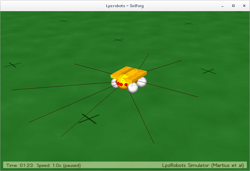
Obstacle Avoidance of a fourwheeled Robot
lpz-Robots simulation with a fourwheeled robot, driving on a playground
and trying to avoid collisions with other objects.
The Task:
Implement the obstacle avoidance feature of the two-wheeled Differential robotcar for a four-wheeled car using infrared (IR) or other type of sensors. Place random obstacles or design a maze to demonstrate its functionality.
Robot Setup
LPZ-Robots is a C++ based package, wich provides classes and functions to physically simulate a robot in a given enviroment. If you want to learn more about lpz-robots, visit their hompage at Uni Leipzig.
In Figure 1 you can see a picture of our robot-setup. We used the \( \texttt{fourwheeled} \) template with the fourwheeled \( \texttt{nimm4} \) robot. We then added the IR sensors and \( \texttt{basiccontroller} \) of the basic example. The complete source code is available in the download section.
We had two ideas to improve the given basic-controller:
The first idea was to integrate a fuzzy logic
to the control-sequencies in order to make the movement of the robot smoother and let it appear more natural.
Our second idea was called 'vector controller'. You will find more details in the corresponding sections of this documentation.
The If Controller
At first we made the robot work with a very simple controller that uses if-else clauses to decide wether to turn left/right or go straight ahead.
Here is the slightly modified code of the \( \texttt{basiccontroller} \):
if (sensors[SIdx("IR front left")] > threshold_backward &&
	sensors[SIdx("IR front right")] > threshold_backward) {
  // move backward if something's in front of the robot
  motors[0] = -.5; // right motor
  motors[1] = -.5; // left motor
}
else if (sensors[SIdx("IR left")] > threshold_sides ||
	 sensors[SIdx("IR front left")] > threshold ||
	 sensors[SIdx("IR front left left")] > threshold_front_sides) {
  // turn right if something's on the left side
  motors[0] = -.25; // right motor
  motors[1] = .75;  // left motor
}
else if (sensors[SIdx("IR right")] > threshold_sides ||
	 sensors[SIdx("IR front right")] > threshold ||
	 sensors[SIdx("IR front right right")] > threshold_front_sides) {
  // turn left if something's on the right side
  motors[0] = .75;  // right motor
  motors[1] = -.25; // left motor
}
else {
  // else move forward
  motors[0] = 1.; // right motor
  motors[1] = 1.; // left motor
}
With the different thresholds \( \texttt{threshold} \), \( \texttt{threshold_front_sides} \), \( \texttt{threshold_sides} \) and \( \texttt{threshold_backward} \) we can change the sensitivity of the different IR sensors. The sensors return values between \( 0 \) and \( 1 \), where \( 0 \) means no obstacle in range of the sensor and \( 1 \) means there is something right in front of it. The robot is steered like a tank, wich is the reason why we have only two different motorspeed values \( \texttt{motors[0]} \) and \( \texttt{motors[1]} \).
In Video 1 one can see the behaviour of the robot with the simple If Controller. Figure 2 shows more precisely the arrangement of the IR-sensors.

As you can see in Video 1, the If Controller works quite well in the choosen \( \texttt{Corridor} \) playground: The robot does not collide with the walls and finds its way through the corridor.
Notation
For reasons of simplification, one can introduce some symbols representing the used variables and assignments in Codebox 1. The vector \( \vec{M} = \left( \texttt{motors[0]}, \ \texttt{motors[1]} \right)^T \) represents the actual motor values at a given point in time. The vectors \( \vec{M}_i \), with \( i \in \{ 1, 2, 3, 4 \} \) represent the four different modes of movement (cf. Codebox 1): \begin{align} \vec{M}_1 &= \left( \begin{matrix} - 0.5 \\ - 0.5 \end{matrix} \right) \nonumber \\ \vec{M}_2 &= \left( \begin{matrix} - 0.25 \\ + 0.75 \end{matrix} \right) \nonumber \\ \vec{M}_3 &= \left( \begin{matrix} + 0.75 \\ - 0.25 \end{matrix} \right) \nonumber \\ \vec{M}_4 &= \left( \begin{matrix} + 1.0 \\ + 1.0 \end{matrix} \right) \ , \\ \end{align} where \( \vec{M}_1 \) represents the backward, \( \vec{M}_4 \) the forward movement, \( \vec{M}_2 \) a turn to the right and \( \vec{M}_3 \) a turn to the left.
The assignment of a value, that corresponds to a `\( \texttt{=} \)` in the Code, will in the following be denoted by the mathematical symbol \( \mapsto \). The idea of replacing the if structure in Codebox 1 by sigmoid functions is based on the fact, that in principle one can rewrite the code in the following way: $$ \vec{M} \quad \mapsto \quad \sum_{i=1}^4 c_i \vec{M}_i \ , \label{eq:assignment_motor_values}$$ where \( c_i \) with \( i \in \{ 1, 2, 3, 4 \} \) are prefactors that mirror the behaviour and hierarchy of the if queries used in the If Controller, i.e. they are \( c_i = 1 \), corresponding to the truth value True, if condition \( i \) is met and the others are not and \( c_i = 0 \), corresponding to False, otherwise. As the hierarchy of if queries should be the same as in the If Controller, there is always only one of the \( c_i \)'s that is equal to \( 1 \), the other ones beeing equal to \( 0 \).
In the next two sections there is a detailed description of how \( c_i \)'s can be calculated with the help of Heaviside functions, in order to get a controller equal to the If Controller. When one has found a proper way of representing the \( c_i \)'s with Heaviside functions, one can simply replace the Heaviside functions with sigmoid functions, that allows the \( c_i \)'s to be in the interval \( c_i \in [ 0, 1 ]\) and hence, enables the mixing of different modes of movement and a smooth transition between those modes. As the \( c_i \)'s in this case are no binary truth values any more, they resemble the idea of continuous truth values that appear in the so called Fuzzy Logic. Each \( c_i \) is then a continuous measure of how True or False an if query is.
Sigmoid Controller
Boolean algebra with Heaviside functions
In order to introduce a smooth transition between the different modes, in a first step the upper code (Codebox 1) for the If Controller with several if blocks was reformulated with the help of the Heaviside function \( \Theta (x) \), for which $$ \Theta(x) = \begin{cases} 1 &\mbox{if } \ x \geq 0 \\ 0 &\mbox{otherwise } \end{cases} \label{eq:heaviside}$$ holds true.
When one defines the integer 1 as True and the integer 0 as False, one can write all if queries of the type $$ a \geq b \quad \Leftrightarrow \quad a - b \geq 0 $$ as $$ \Theta(a-b) \ . $$ As \( \Theta (x) \) only takes the values 0 or 1, one can use basic algebra in order to formulate the boolean operation A AND B, in the following denoted by \( A \wedge B \), where \(A = \Theta(a)\) and \(B = \Theta(b)\) are logic values, as a multiplication of \( \Theta \) functions: \begin{equation} \text{AND:} \quad A \wedge B \quad \hat{=} \quad \Theta(a) \cdot \Theta(b) \ . \label{eq:and} \end{equation}
The boolean operation NOT A, which in the following will be denoted as \( \lnot A \) can be translated into the Heaviside representation as follows: \begin{equation} \text{NOT:} \quad \lnot A \quad \hat{=} \quad \Theta(-a) \ . \label{eq:not} \end{equation} However, there is a problem at \( a = 0 \), as for the given definition of the Heaviside function from Equation (\ref{eq:heaviside}), it is \( \Theta(- 0) = \Theta(0) = 1 \). On the other hand, for \( a = 0 \) it is \( A = \Theta(a) = 1 \) and therefore \( \lnot A = 0 \). Accordingly, Equation (\ref{eq:not}) only holds true for \( a \neq 0 \). With this subtlety in mind, one can go on and check, how the logical operation A OR B could look like, when written with Heaviside functions.
The logical A OR B operation, in the following denoted as \( A \vee B \), can, according to basic boolean algebra, be written as $$ A \vee B \quad = \quad \lnot \left\{ \left( \lnot A \right) \wedge \left( \lnot B \right) \right\} \ , $$ and hence, can be reduced to the already discussed operations AND and NOT. However, due to the aforementioned subtlety, that causes \( \Theta(\Theta(x)) \neq \Theta(x) \) for values of \( x < 0 \), it is no good idea to do nesting of Heaviside functions in order to compute truth values. It turns out, that there is another reason concerning the later discussed replacement of Heaviside with sigmoid functions, that turns the nesting into a bad idea.
However, there is a different representation of \( A \vee B \) that proofs helpful: $$ A \vee B \quad = \quad \left( A \wedge B \right) \quad \vee \quad \left( (\lnot A) \wedge B \right) \quad \vee \quad \left( A \wedge (\lnot B ) \right) \ . \label{eq:or_repr} $$ From the first sight, Equation (\ref{eq:or_repr}) only turns one OR expression into two. However, we know that in any case, either one or none of the three terms is True, while the others are False. Hence, in terms of Heaviside functions, we can simply write the OR operation as follows: \begin{equation} \text{OR:} \quad A \vee B \quad \hat{=} \quad \Theta(a) \cdot \Theta(b) \quad + \quad \Theta(-a) \cdot \Theta(b) \quad + \quad \Theta(a) \cdot \Theta(-b) \ . \label{eq:or} \end{equation} Note that the algebraic representation of OR as \( + \) is not directly applicable to \( A \) and \( B \), in the sense, that $$ A \vee B \quad \neq \quad \Theta(a) + \Theta(b) \ . \label{eq:wrong_or} $$ The right hand side of Equation (\ref{eq:wrong_or}) is not limited to the values 0 and 1, as when both \( A \) and \( B \) are True, we have \( 1 + 1 = 2 \). With nesting the result into another Heaviside function, this problem could be solved, however the nesting ought to be avoided here.
Additionally to the boolean operations AND and OR and their representations in terms of Heaviside functions from equations (\ref{eq:and}) and (\ref{eq:or}) one needs to find representations for the counterparts NAND and NOR, that get along without nesting of Heaviside functions. After the discussions above, these representations can be found straightforward as: \begin{align} \text{NOR:} \quad \lnot (A \vee B) = (\lnot A) \wedge (\lnot B) \quad &\hat{=} \quad \Theta(-a) \cdot \Theta(-b) \\ \text{NAND:} \quad \lnot (A \wedge B) = (\lnot A) \vee (\lnot B) \quad &\hat{=} \quad \Theta(-a) \cdot \Theta(-b) \quad + \quad \Theta(a) \cdot \Theta(-b) \quad + \quad \Theta(-a) \cdot \Theta(b) \ . \end{align}
Now we have all expressions we need, to find the correct expressions for \( c_i \)'s. The details on this can be found in the next section.
Replacing if clauses by Heaviside formalism
All logical queries of the If Controller (cf. Codebox 1), are of type $$ S - T > 0 , \label{eq:basicineq}$$ where \( S \) is some sensor value and \( T \) the corresponding threshold. It makes little to no difference for the controller, whether there is a \( > \) or a \( \geq \) in Inequality (\ref{eq:basicineq}). Therefore, the corresponding truth value for Inequality (\ref{eq:basicineq}) will be calculated by \( \Theta(S-T) \), although the above definition of \( \Theta(x) \) uses the \( \geq \) sign.
In Codebox 2 the result of above discussions in terms of a programm code for the Heaviside Controller is presented. Variables \( \texttt{A1, A2, A3, B1, B21, B22, B31, B32} \) are auxiliary variables storeing the left hand side of Inequality (\ref{eq:basicineq}) for all sensors and their corresponding thresholds. These auxiliary variables are the arguments of the Heaviside function, which is here calculated via the function \( \texttt{double activation(double x)} \). The results of the Heaviside function are then used in order to apply the obtained expressions for logical operations from the preceding section and therefore calculate the truth values for Conditions 1, 2, 3 and store them in \( \texttt{C1, C2, C3} \). The variables \( \texttt{NOTC1, NOTC2, NOTC3} \) are calculated according to the same algebraic expressions of logical operators and represent the negations of \( \texttt{C1, C2, C3} \).
In the last few lines of Codebox 2 the proper motor values are calculated from \( \texttt{C1, C2, C3} \) and \( \texttt{NOTC1, NOTC2, NOTC3} \) and are assigned to \( \texttt{motors[0]} \) and \( \texttt{motors[1]} \). The hierarchy of if queries from the If Controller is hereby preserved, due to the following correspondence: \begin{align} c_1 &= \texttt{C1} \nonumber \\ c_2 &= \texttt{NOTC1} \cdot \texttt{C2} \nonumber \\ c_3 &= \texttt{NOTC1} \cdot \texttt{NOTC2} \cdot \texttt{C3} \nonumber \\ c_4 &= \texttt{NOTC1} \cdot \texttt{NOTC2} \cdot \texttt{NOTC3} \ , \end{align} where \( c_i \ , i \in \{1, 2, 3, 4\} \) refers to the prefactors that were introduced above. With this correspondence the assignments of motor values simply follows Equation (\ref{eq:assignment_motor_values}).
It is noteworthy to mention, that in some cases, when one of the arguments of the Heaviside function is exactly equal to \( 0 \), there might be some strange behaviour, as \( \texttt{C1, C2, C3} \) and \( \texttt{NOTC1, NOTC2, NOTC3} \) are no longer truth values. They might get greater than \( 1 \) and it is possible, that \( \texttt{NOTC1, NOTC2, NOTC3} \) is no longer the negation of \( \texttt{C1, C2, C3} \). There are two reasons why this problem can be ignored. The first reason beeing, that the frequency and duration of this problem happening during the simulation is negligible. The second reason is, that the Heaviside function gets replaced by the sigmoid function anyways. The hypothesis, that the problem can be ignored is supported by the fact, that no difference in the behaviour of the robot when switching between If Controller and Heaviside Controller can be observed.
// auxiliary variables; arguments of Heavisides
double A1, A2, A3;
double B1, B21, B22, B31, B32;

double C1, C2, C3;             // Conditions 1, 2, 3
                               // (results of algebraic representation of logical operators as Heavisides)
double NOTC1, NOTC2, NOTC3;    // Negations of Conditions 1, 2, 3


// ------------ Condition 1 ------------
A1    = sensors[SIdx("IR front left")] - threshold_backward;
B1    = sensors[SIdx("IR front right")] - threshold_backward;

// C1 = A1 AND B1
C1    = activation( A1) * activation( B1);
NOTC1 = activation(-A1) * activation( B1) +
        activation( A1) * activation(-B1) +
        activation(-A1) * activation(-B1)


// ------------ Condition 2 ------------
A2    = sensors[SIdx("IR left")] - threshold_sides;
B21   = sensors[SIdx("IR front left")] - threshold;
B22   = sensors[SIdx("IR front left left")] - threshold_front_sides;

// C2 = A2 OR B21 OR B22
C2    = activation( A2) * activation(-B21) * activation(-B22) +
        activation(-A2) * activation( B21) * activation(-B22) +
        activation(-A2) * activation(-B21) * activation( B22) +
        activation( A2) * activation( B21) * activation(-B22) +
        activation( A2) * activation(-B21) * activation( B22) +
        activation(-A2) * activation( B21) * activation( B22) +
        activation( A2) * activation( B21) * activation( B22);
NOTC2 = activation(-A2) * activation(-B21) * activation(-B22);


// ------------ Condition 3 ------------
A3    = sensors[SIdx("IR right")] - threshold_sides;
B31   = sensors[SIdx("IR front right")] - threshold;
B32   = sensors[SIdx("IR front right right")] - threshold_front_sides;

// C3 = A3 OR B31 OR B32
C3    = activation( A3) * activation(-B31) * activation(-B32) +
        activation(-A3) * activation( B31) * activation(-B32) +
        activation(-A3) * activation(-B31) * activation( B32) +
        activation( A3) * activation( B31) * activation(-B32) +
        activation( A3) * activation(-B31) * activation( B32) +
        activation(-A3) * activation( B31) * activation( B32) +
        activation( A3) * activation( B31) * activation( B32);
NOTC3 = activation(-A3) * activation(-B31) * activation(-B32);


// ------------ Assign Motor values ------------
//          backward +  turn right      +  turn left             + forward
motors[0] = -0.5*C1  +  (-.25)*NOTC1*C2 +  ( .75)*NOTC1*NOTC2*C3 + 1.0*NOTC1*NOTC2*NOTC3;   // right motor
motors[1] = -0.5*C1  +  ( .75)*NOTC1*C2 +  (-.25)*NOTC1*NOTC2*C3 + 1.0*NOTC1*NOTC2*NOTC3;   // left motor
Replacing Heaviside with sigmoid function
The sigmoid function \( \text{sig}(x) \) is defined as follows: \begin{equation} \text{sig}(x) = \frac{1}{1 + \exp\left\{-s\left(x-b\right)\right\}} \quad \in [0, 1] \ , \end{equation} where \( s \) determines the slope of the transition between \( 0 \) and \( 1 \) and \( b \) is a bias that shifts the function along the \( x \) axis. In our project we found \( b = 0.05 \) and \( s = 10.0 \) to be suitable. The function \( \text{sig}(x) \) for these parameters can be seen in Figure 3.
In the downloadable code \( b \) corresponds to the variable \( \texttt{bias} \) of the \( \texttt{activation} \) function and \( s \) corresponds to the parameter \( \texttt{slope_sigm} \) that can be changed during runtime. The behaviour of the \( \texttt{activation} \) function either being a Heaviside or a sigmoid function can be changed during runtime by the boolean variable \( \texttt{heaviside} \). To switch from the If Controller to Heaviside or Sigmoid Controller one can set the runtime parameter \( \texttt{use_if} \) to \( 0 \).
First thing to notice when investigating the behaviour of the robot for the Sigmoid Controller, is the smooth transition to the Heaviside Controller, when taking the limit of \( s \rightarrow \infty \). In this limit we easily see, that the variable \( b \) only shifts our previously introduced threshold \( T \). When \( s \) takes a finite value, \( b \) determines the point where \( \text{sig}(x=b) = \frac{1}{2} \). Additionally, \( b \) determines how much \( \text{sig}(x) \) and \( \text{sig}(-x) \) overlap and is therefore important when the logic negation operation is calculated - cf. Equation (\ref{eq:not}).
As mentioned previously the nested versions of algebraic expressions for truth value calculation is a bad idea when using Heaviside functions. This also holds true for the Fuzzy Logic with sigmoid functions: The result of the sigmoid function is strictly in the interval \( \text{sig}(x) \in [0, 1] \), while the result for nested sigmoid functions only makes up subintervalls of \( [0, 1] \), e.g.: \( \text{sig}(\text{sig}(x))\Big\vert_{b=0} \in [0.5, \text{sig}(1)] \). This issue can in principle be solved by rescaling the outcome of the inner sigmoid function. However, here the solution of avoiding nested Heavisides and sigmoids was chosen instead.
The \( \texttt{activation} \) function allows via the boolean variable \( \texttt{heaviside} \) to switch between Heaviside and sigmoid output during runtime. Accordingly the code for the sigmoid controller remains unchanged compared to the heaviside controller, except for a small change in the assignment of motor values. The values \( \texttt{C1, C2, C3} \) and \( \texttt{NOTC1, NOTC2, NOTC3} \) for the Heaviside case are either \( 0 \) or \( 1 \), which allows the controller to use the full range of possible motor values from the interval \( [-1, 1] \). For the Sigmoid Controller the motor values tend to be in a smaller interval, which makes the robot drive more slowly. In order to address this problem, the motor values were mapped to the interval \( [-1, 1] \) via a \( \tanh(x) \) function with a suitable slope of \( \texttt{slope_tanh} = 25.0 \) - cf. Codebox 3.
// ------------ Assign Motor values ------------
//                           backward +  turn right      +  turn left             + forward
motors[0] = tanh(slope_tanh*(-0.5*C1  +  (-.25)*NOTC1*C2 +  ( .75)*NOTC1*NOTC2*C3 + 1.0*NOTC1*NOTC2*NOTC3));   // right motor
motors[1] = tanh(slope_tanh*(-0.5*C1  +  ( .75)*NOTC1*C2 +  (-.25)*NOTC1*NOTC2*C3 + 1.0*NOTC1*NOTC2*NOTC3));   // left motor
In Video 2 one can see the comparison between the If Controller that causes a jittering movement and the smooth movements of the robot for the Sigmoid Controller. As expected the behaviour of the robot is in principle the same, however, the transition between the different modes of movements is smooth for the Sigmoid Controller.

Vector Controller
We also thought about a completely different approach to design a controller. Our robot perceives his environment only through the infrared sensors, attached around his body. The idea was to "draw a mental picture" of the environment measured by the sensors and then head in the direction where most likely is no obstacle blocking the way.
To know which direction is safe to go, a vector is calculated, that points in the direction of the - on average - largest distance to surrounding obstacles, calculated by the sensor data. In Codebox 4 the components of the vector \( \vec{V} = ( \texttt{vecx},\texttt{vecy} )^T \) are calculated and assigned to the motors.
// computing the x- and y- components of the vector
double vecx =  - 1.0 *(1-sensors[SIdx("IR left")])            - 0.7*(1-sensors[SIdx("IR front left left")])
	       - 0.15*(1-sensors[SIdx("IR front left")])      - 0.3*(1-sensors[SIdx("IR back left")])
	       + 0.15*(1-sensors[SIdx("IR front right")])     + 0.7*(1-sensors[SIdx("IR front right right")])
	       + 1.0 *(1-sensors[SIdx("IR right")])           + 0.3*(1-sensors[SIdx("IR back right")]) ;

double vecy =    0.7 *(1-sensors[SIdx("IR front left left")]) + 0.98*(1-sensors[SIdx("IR front left")])
               + 0.98*(1-sensors[SIdx("IR front right")])     + 0.7 *(1-sensors[SIdx("IR front right right")])
               - 1.68*(1-sensors[SIdx("IR back left")])       - 1.68*(1-sensors[SIdx("IR back right")]) ;

// set the motor values
motors[0] = base_speed + vecy - vecx; // right motor
motors[1] = base_speed + vecy + vecx; // left motor
As mentioned earlier, an IR sensor returns \( 1 \) when an obstacle is right in front of it. To obtain a vector, pointing in the opposite direction of the obstacle, we use \( \texttt{ 1-sensors[SIdx("IR ...")] } \). For \( \texttt{vecx} \) the prefactors of the sensor values are a result of simple vector-algebra: The \(x\) component of e.g. \( \texttt{IR front left} \) is: \( v_x^{\text{FL}} = \sin(\pi / 20) = 0.15 \) (cf. Figure 4). It is required that \( \vec{V} = (0,0)^T \), when there is no obstacle around the robot (in the range of the IR sensors), i.e. when all sensors return \(0\). This works well for \( \texttt{vecx}\), since the arrangement of the sensors is symmetrical to the \(y\) axis.
As for \( \texttt{vecy} \) the arrangement of the sensors is not symmetrical to the \(x\) axis, but we still demand \( \vec{V} \) to be \(\vec0\), when no obstacle is around, the two back sensors have to cancel out the front sensors, so their prefactors are adjusted to be the sum of the front sensors.
To let the robot go forward, when no obstacle is around, we set the \( \texttt{ base_speed } \) variable. Its default value is \(1\) and it is modifiable at runtime.

A little flaw of this controller occurs, whenever \( \vec{V} = ( 0 , -\texttt{ base_speed } )^T \) is met. Then both, \( \texttt{motors[0]} \) and \( \texttt{motors[1]} \) become \( 0 \) and the robot gets stuck. This can be observed in Video 5.
Comparison of all controllers
In Video 4 and 5 one can see the behaviour of the robot for all discussed controllers in a different playground called \( \texttt{SquareGround} \) either with or without random obstacles. Due to the hierarchical structure for the different modes of movement for both If and Sigmoid Controller a turn to the right is not equitable compared to a turn to the left. This can be observed especially in Video 4.
In Video 5 obviously for both If and Vector Controller the robot tends to get stuck at some stage. Concerning the If Controller one can again observe the jittering movement when switching between different modes of movement at a high obstacle density. In turn the Vector Controller gets stuck whenever \( \vec{V} = (0, -\texttt{base_speed})^T \).
However, there is also a drawback for the Sigmoid Controller: When the obstacle density is too high the robot often doesn't fulfill the task of avoiding obstacles and instead bumps into them and pushes them out of the way. This issue might be solvable by using more sensors around the robot or by finetuning the existing thresholds.