Intelligent Driver Model in LpzRobots
- A simulation of self organization in closed traffic lines -
AbstractIn 2008 an experimental evidence for the physical mechanism of forming a jam [1] was published, amongst others showing the dynamics of a closed traffic line (see here). Encouraged to generate such and more behaviour in the LpzRobots simulation [4] we reproduced the experimental set-up using a simple model that reduces the number of parameters to be manageable but still captures the behaviour of a real-life driver. We find these requirements satisfied in the Intelligent Driver Model [2]. Note that we don't want a model that suites for real life driver assistance but one that is simple to examine. |
Content |
The Intelligent Driver Model
Overview
The Intelligent Driver Model (IDM) is a time-continuous car-following model for the simulation of freeway and urban traffic, which was developed by Treiber, Hennecke and Helbing in 2000 [3].The model comes with a wide range of adjustable parameters. In order to calculate the IDM for one vehicle (i.e. its new velocity) information about its current velocity $v$ and its distance to the vehicle in the front $s$ just as about the their velocity difference $\Delta v$ is needed.
Equation And Parameters
The differential equation of the Intelligent Driver Model is given by the following formula: $$ \begin{array}{rcl} \dfrac{dv}{dt} = a\left[ 1-\left( \dfrac{v}{v_{0}}\right)^{\delta}-\left(\dfrac{s^{*}(v,\Delta v)}{s}\right)^{2}\right] \\ \end{array} $$ $$ \begin{array}{rcl} s^{*}(v, \Delta v) = s_{0}+vT+\dfrac{v\Delta v}{2\sqrt{ab}} \end{array} $$ where- $v_{0}$: Velocity which the vehicle would drive on a free road.
- $s_{0}$: Minimal distance to the vehicle in front.
- $T$: Desired safety time headway to the vehicle in front.
- $a$: Acceleration.
- $b$: Comfortable braking deceleration.
- $\delta$: Acceleration exponent.
Behaviour Of The Differential Equation
The IDM consists of the first term, which determines the acceleration of the vehicle on a free road, and a second one for the deceleration in case of traffic ahead.
When the way is nearly free the distance $s$ to the vehicle in front is high and therefore the second term gets insignificant. Additionally, the acceleration term gets zero when a vehicle reaches its desired velocity $v_{0}$. On the other hand the acceleration limits 0 when the actual distances $s$ approaches the value of the desired distance $s^{*}$ because $v$ is 0.
One of the most important parts of the IDM is the term determining $s^{*}$, which amongst others is characterized by the desired safety time $T$. The term increases if the vehicle in front comes closer to a slower one and decreases if it moves away.
Behaviour Of Traffic Flow
To analyse the flow of traffic, we first search for equilibrium states. For that we set $$ \begin{array}{rcl} \dfrac{dv}{dt}=0 \end{array} $$ This can be satisfied if all cars move with the same velocity $v'$ with a fixed distance $s'$. For cars on a circle, this distance is determined by the Radius of the circle $r$ and the number of cars N. $$ \begin{array}{rcl} s'=\dfrac{2\pi r}{N} \end{array} $$ We find that there must be one positive $v'$ that satisfies this condition, but it cannot be determined analytically. Here are some numeric values for the parameters $s_{0} = 3.0$, $a = 4.5$, $b = 4.0$, $\delta = 4$, $T = 0.5$, $r = 35.5$, $N = 30$:
| $v_{0}$ | $v'$ |
|---|---|
| 4.0 | 3.328 |
| 4.5 | 3.666 |
| 5.0 | 3.984 |
| 5.5 | 4.281 |
| 6.0 | 4.557 |
| 6.5 | 4.812 |
| 7.0 | 5.045 |
| 7.5 | 5.257 |
| 8.0 | 5.449 |
This is the maximal velocity a car can reach for a given set of parameters.
Implementation
Basic Functions
All code parts of the simulation are linked at the bottom of this page. This section gives a short overview about the ideas behind out programm.
To create a collective movement along a circle the two wheels of each robot are of different size. When the simulation gets started the robots are placed successiveley in a distance relating to the total number of robots along a circle of suitable radius. The correct orientation is achieved by a extension of the Differential constructor. Furthermore the robots can be positioned on only a percentage of the circle range.
In this simulation the IDM differential equation is solved for every time step (0.01 s) for every robots by the euler method, which calculates the new postion and new velocity. The ODE has in principle the following form and can therefore be distinguished as coupled: $$ \begin{array}{rcl} \dfrac{dx}{dt} &=& v \\ \dfrac{dv}{dt} &=& f(v) \end{array} $$
Instead of implementing different kind of robots with different parameters we use a global noise in the controller unit to produce diverse dynamics.
The distance between a robot and that in front is measured by a Infra-red-sensor (IR-sensor) on the front side. Due to its behavior the variables of the IDM equation had to be modified in a appropiate manner:
v = wheelcorr * maxSpeed * motors[MIdx("right motor")];
dx = IRrange * (1 - sensors[SIdx("IR front left")]);
dv = (dxOld - dx) / 0.01;
The IDM
if (sensors[SIdx("IR front left")] == 0)
{
	double deriv = a * (1 - pow((v / v0), delta));
	motors[MIdx("right motor")] = (v + deriv * 0.01) / (wheelcorr * maxSpeed);
	motors[MIdx("left motor")] =  (v + deriv * 0.01) / (wheelcorr * maxSpeed);

}

else
{
	double deriv = a * (1 - pow((v / v0), delta)- pow((sDesired / dx), 2));


	if ((v + deriv * 0.01) / (wheelcorr * maxSpeed) < 0)
	{
		motors[MIdx("right motor")] = 0;
		motors[MIdx("left motor")] =  0;
	}

	else
	{
		motors[MIdx("right motor")] = (v + deriv * 0.01)  / (wheelcorr * maxSpeed);
		motors[MIdx("left motor")] =  (v + deriv * 0.01) / (wheelcorr * maxSpeed);
	}
}
To adapt the differential equation to the simulation we added if..else-statements. The first one ensures that the robot shows "free traffic behavior" when the sensor value is 0, though to the normalization. With the second statement the velocity can never be smaller than 0. This guarantees that the simulation runs stable, even if the initial distance between the robots is smaller than the minimum distance $s_{0}$.
main.cppdifferential.cpp
basiccontroller.cpp
differential.h
Project Code
Here you can download the project file of the simulation as a zip-folder.
Experiments and Results
To give some impression of the actual behaviour of the robots you can look at the two following videos. The first one is without noise, the second one is with noise set to 0.125. These are the same parameter settings analysed in Section 1 of Experiments and Results.
Analysis of a single experiment
Note: you can enlarge every image by clicking.To develop analysis tools for circular traffic jams, we first had a look at one single experiment with following parameters:
- $v_{0}$: 4 m $\cdot$ s$^{-1}$
- $s_{0}$: 4 m
- $T$: 0.5
- noise: 0.0

The average velocity of all robots (Fig. 1a) seemed to be a good estimate for "effiency" while driving in a jam.
1a) mean velocity of all cars

The velocities of single cars are too complex and need further analysis, which you can see in Fig. 1h. The same argument holds for the distance to the following robot (Fig. 1d), here plotted for 3 robots.
1b) velocity of first three cars

1c) distance to previous car

The standard deviations of both velocity and distance to next robot seem to be measures of the severeness of the traffic congestion.
1d) standard deviation of velocities

1e) standard deviation of distance to previous car

Of highly interest was the travelled distance in total in relation to time. The plot shows increasing and decreasing distances to other cars plus the average travelling of all cars. One could say, it combines the plots of every single velocity and distance. The travelled distance was obtained by integrating over velocity.
1f) travelled distance in time
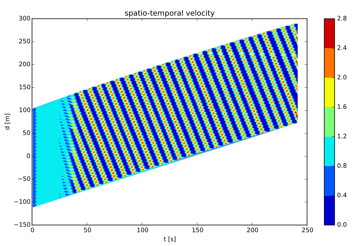
As shown in the plot "travelled distance - time", there seem to be some "stop and go waves" in the system, which can be investigated further. Therefore a velocity dimension is added and a spatial-temporal velocity profile is obtained. This intuitive shows the wave-like behaviour.
1g) spatio temporal velocity profile

To determine the features of the stop and go waves, a Fast-Fourier-Analysis with the Hanning-window function of the velocity was performed. The sampling rate was 20 Hz (the Nyquist-sampling-Theorem therefore delivers a maximal frequency of 10 Hz), but one can assume that realistic waves have a frequency below 2Hz. The velocity of a wave was obtained from the time shift between the signals of following cars.
1h) Fourier-Analysis

Plotting the angle in the roundabout versus the velocity of one car allows the investigation of a transformed phase-space. The obtained "flower-pattern" is a common features of traffic congestion.
1i) Angle - Velocity Space
Variation of both desired velocity and noise
To investigate the influence of the velocity on the self-organisation of a traffic congestion and how the system behaves with or without noise, we varied both paramters.

For the given set of parameters (s0 = 4m) we state that increasing the maximal velocity also increases the velocity of all cars. If the safety distance to another car is large, it seems better to drive faster. Then the traffic congestion itself moves faster.
2a) Average velocity

The standard deviation of the distance shows, that once a traffic congestion is reached, the system won't go back to a laminar phase. In contrast, there are some maximal velocities, where there is no traffic congestion in simulation time. With the given noise, a congestion will form.
2b) Standard deviation of distance
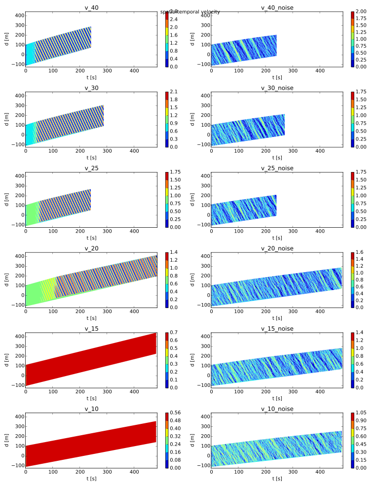
With decreasing velocity, it takes longer to self-organise into a traffic congestion. For small velocities, a truly laminar phase is reached, as described above.
2c) Spatio-temporal velocity
Variation of Noise for fixed maximal velocity
The following plots show the influence of noise on the development of a traffic congestion. For global noise set to 0, there is only a laminar phase. We find a criticial noise level, where a traffic congestion forms. The lower the noise, the longer it takes to reach this phase.

The average velocity of the cars in a traffic congestion drops with increasing noise.
3a) Average Velocity

For increasing noise-levels, the stop and go waves are getting continous,so the waves are no longer discriminable.
3b) Travelled distance - time
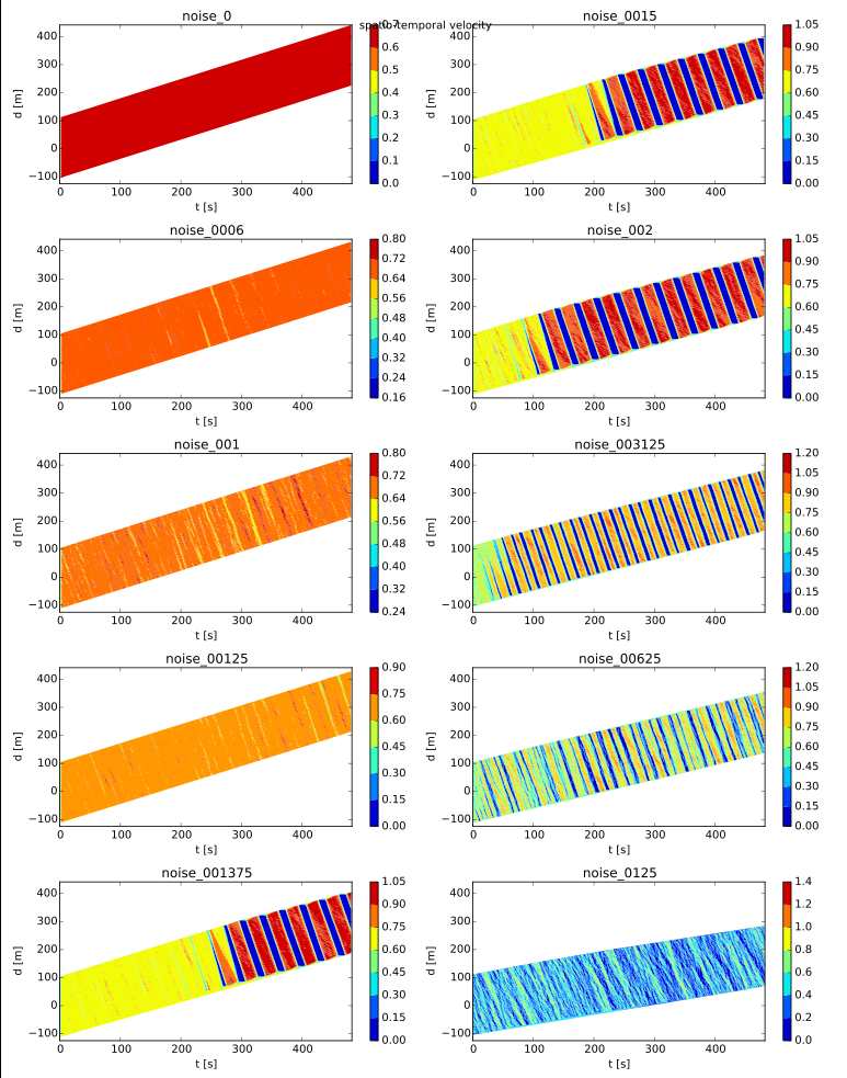
The velocity profile shows a similar trend as Figure 3b.
3c) spatio-temporal velocity profile
Variation Percentage initial position
The following analysis shows how the system can compensate small levels of perturbation. The perturbation was implemented with a Circle-Percentage, which describes, how much of the circle was used to initialise all robots. (Determines the interval of starting phases [0, 2*pi * factor]).

The spatial-temporal velocity shows, that the system can compensate a perturbation of 0.98. Above this value, a stable laminar phase is reached, below the system organises into a traffic congestion.
4a) spatio-temporal velocity profile
Decreased safety distance
In the following experiment, the influence of the safety distance $s_{0}$ was investigated. The only change to the first experiment is the safety distance (from 3 m to 4m). We choose different velocity intervals because of the changed dynamics.

With increased maximal velocity, the average velocity drops. If you drive close to the following car, it is better for the group to desire a slower speed.
5a) Average Velocity

The results of a change in safety distance are also shown here. Decreased safety distance leads to a higher average velocity, but increasing velocity for a smaller safety distance leads to decreasing average velocity.
5b) Comparison of average velocity in congestion in dependency from maximal velocity and safety distance
Conclusions
We therefore conclude several advises for drivers how to avoid a traffic congestion or how to be most efficient in a congestion:
- Drivers should stay concentrated to have a minimal level of noise (a higher attention and concentration level). If global noise is lower, it is more likely to avoid traffic congestions for the whole group.
- Drivers can risk to reduce the distance to the next car in trade-off with a slower maximal velocity. This behaviour increases the overall velocity of the traffic congestion.
- Drivers should not try to go as fast as possible when accelerating. Lower velocities have a higher chance to not get into a traffic congestion and have higher capabilities of compensating noise.
Authors
- Tim Koglin, bachelor student
- Nicklas Riebsamen, bachelor student
- Sigrid Trägenap, bachelor student
Sources & References
We want to especially thank Laura Martin, Bulcsú Sándor & Hendrik Wernecke for the proposal of the topic and their continous support during its development.
- "The Mathematical Society of Traffic Flow", Yuki Sugiyama et al., New Journal of Physics, 2008, Multimedia supplement.
- Treiber, M.; Hennecke, A. und Helbing, D.: Congested traffic states in empirical observations and microscopic simulations, Physical Review E 62 (2000), pp. 1805–1824.
- Wikipedia
- LPZ Robot Package & its documentation Intelligent driver model
Legal note: We do not take any responsibility for the content of the webpages linked here.
Page design inspired by Hellfrisch, Born, Beberweil.