Biham-Middleton-Levine traffic model
An applet of a cellular automaton
Abstract
The Biham-Middleton-Levin model is a simple system to simulate traffic within a city. It consists of two types of agents (called cars) that can either move down (red) or right (blue). The traffic is controlled by traffic lights, so that in each time step only one type can move. The agent will not move, if it is blocked by an agent of different type or by an agent of the same type which is blocked itself. The system underlies periodic boundary conditions and the characteristics of the system is mainly determined by the density of agents and the random initial conditions. For a low density one will find a free flowing phase (e.g. system size $100$, density $20\%$), where no agent is blocked. For larger densities, a blocked phase (e.g. system size $100$, density $40\%$) is created, so that every agent is blocked. These phases can be observed after a transient period, which is determined by the system size, density and other parameters.
Simulation
Usage of the Applet
In the above applet there are two graphic window, the left one showing the simulation of the agents' movements, the right one depicting the percentage of performed movements per type. For the simulation of the Biham-Middleton-Levine model you can change a few parameters in the applet.
- In the section System Mode one can select the Field mode that provides periodic boundary conditions and corresponds to the original model. The Crossing mode has open boundaries and resembles a crossing of pedestrian crowds. New agents are set to the free fields of the income edge randomly at any time step. (Note: every change initialises a new random initial set.)
- The density of agents is the number of agents (each type about the same number) per area. It determines the behaviour of the system and it can only be changed when the simulation is not running. (Note: every change initialises a new random initial set.) Running the Crossing Field mode however the density slider determines, how many new agents enter the edge of the field.
- With the speed bar one can change the speed of the simulation.
- By car speed you change the relative velocity of the cars. Therefore the red cars (v1) will go on moving one cell per time step, the blue cars will only move with higher velocity (v2). (Note: the agent will only jump in a given time step, when there is enough space infront; e.g. for speed v=3 it needs 3 free fields infront.)
- The system size can be choosen out of four predefined settings. It is the number of cells along an edge of the left field. (Note: every change initialises a new random initial set.)
- To start the simulation just choose your prefered settings and press the start button
- To perform only one step of the simulation you can use the arrow button (next to the start button; only works when simulation is not yet running).
- Note: Whenever you change the parameters System Mode, System Size or Density, a new random set will be initialised. These parameters can only be accessed when the simulation is paused.
Theory
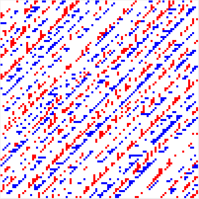
(a) flowing phase system (e.g. system size $100$, density $20\%$)
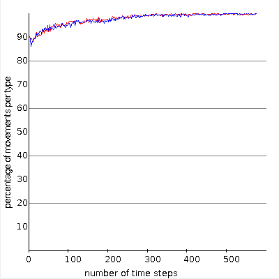
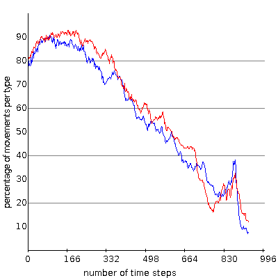
(b) flowing phase statistics
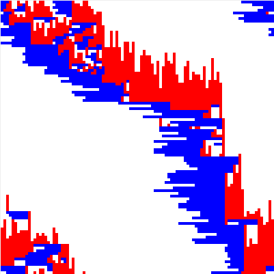
(c) blocked phase system (e.g. system size $100$, density $40\%$)
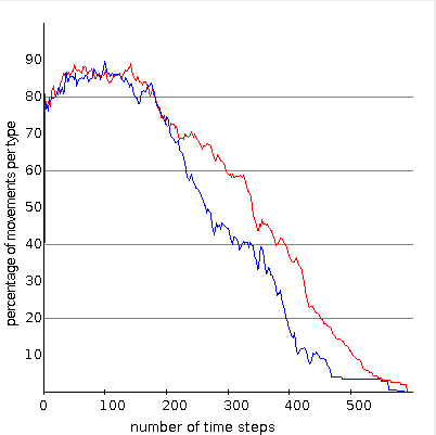
(d) blocked phase statistics
BML Model
The set up for the BML model is a $N\times N$ square lattice of which each node can be either occupied by one agent or is empty. There are two different types of agents characterized by the direction of their movement, which can be seen as cars in the streets of a city. Here one type can move only to the right (blue), the other only moves down (red). The initial configuration of agents on the lattice is a random distribution with an total initial agent density $p$ (ratio of number of all agents with the number of available nodes on the lattice), the probability to find an agent of special type is therefore $p/2$.
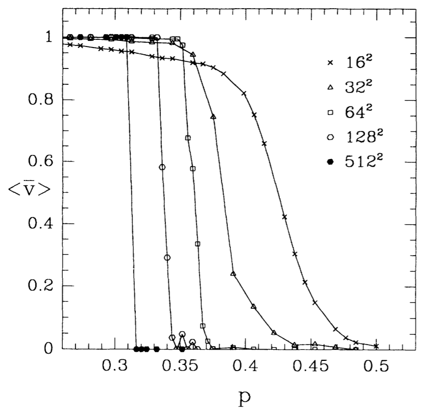
(e) phase transition (from [2])
- If the node infront (in the direction of movement) is empty, it will go there.
- If the node infront is occupied by an agent of the other type, the agent is blocked.
- If the node infront is occupied by an agent of the same type, the agent will move if the infront agent moves.
In the original system proposed in [2] the speed of the agents is limited to one mode per timestep ($v_1=v_2=1$). In the dynamical behaviour Biham et al. find to different asymptotic states. After a transient period which depends on the initial configuraiton and the system size $N$, the agents are either all moving infinitely long without being blocked (flowing phase) or the agents -- all or only a fraction -- is blocked for ever. In Fig. (a) the system is in the free flowing phase and in the corresponding diagramm in Fig. (b) one can see that after a short time all agents are moving. The blocked phase is depicted in Fig. (c) where the typical diagonal structure can be found. There the different types of agents block another and the diagramm Fig. (d) shows that the number of moving agents goes down to zero.
(f) statistics of an unstable intermediate phase going to a locked phase (e.g. system size $100$, density $30\%$)
So the transition between the two extreme states becomes very sharp and the critical density $p_c(N)$ where the transition happens, depends on the system size.
In the original publication the authors compare this second order transition to a percolation transition known from network theory. Up to the very day there is no rigorous analysis of this system except for some special cases of very high density.
Extended Pedestrian Model
This mode was introduced by the authors of this applet and is an extension to the original BML model. The main difference is that the system no longer has periodic boundary conditions but open boundaries. The system starts as before with a random initial distribution of agents of density $p_i$ (both types equally often represented) but whenever an agent leaves the field it is gone. On the entrance edge of each agent type, new agents are created randomly with certain probability $p_n$. To give the system the shape of a pedestrian crossing, some areas (black squares) are forbidden areas for the agents. In this way one can simulate the flow of pedestrians on a crossing when showing the behaviour of the BML model. As the boundaries are no more periodic, there won't be any jams, i.e. the fully blocking phase vanishes.
Code & Documentation
To understand the applet and the way it simulates the given model, the authors share the produced code and a detailled documentation on this.
Available Features
Available Features
- Documentation of the applet. This documentation was created with help of Javadoc and explains the most important parts of the applet.
Javadoc-Documentation of the applet. - Sourcecode of the Applet. This provides a .zip-file containing all Java-files of the applet.
Java-Sourcecode. - Class-files of the Applet. If you can not or do not want to compile the applet, this provides a .zip-file containing all .class-files of the applet.
Class-files.
Acknowledgement, Authors & Contact
Acknowledgement
The authors would like to thank the members of the group Prof. C. Gros for the great help when developing this applet. Especially we thank Prof. C. Gros, Rodrigo Echeveste and Bulcsú Sándor for discussing the model, giving good advice for its visualisation and helping to remove all kinds of technical problems.
About the authors Samuel Eckmann is a Bachelor's student in the group of Prof. C. Gros at Goethe University Frankfurt (Main).
Hendrik Wernecke is a Master's student in the group of Prof. C. Gros at Goethe University Frankfurt (Main). He did his Bachelor studies at Ulm University (2010-2013).
Contact For questions, suggestions or comments on this simulation, please contact wernecke@itp.uni-frankfurt.de.
 Samuel Eckmann
 Hendrik Wernecke
References & Further Reading
- [1]
- Wikipedia article Biham-Middelton-Levine traffic model
- [2]
- : Self-organization and a dynamical transition in traffic-flow models, Phys. Rev. A 46, R6124(R), November 1992.
- [3]
- : Complex and Adaptive Dynamical System - A Primer, Springer-Verlag, 2011.
Legal note: We do not take any responsibility for
the content of the webPages linked here-in.